
A Novel 2.5D Shadow Calculation Algorithm for Urban Environment
Sukriti Bhattacharya, Christian Braun and Ulrich Leopold
Department for Environmental Research and Innovation (ERIN), Luxembourg
Luxembourg Institute of Science and Technology (LIST), Luxembourg
Keywords:
2.5D Shadow, Tensorflow, Bresenham’s Algorithm.
Abstract:
This paper proposes a novel efficient algorithm to calculate a 2.5D shadow map based on a coherent math-
ematic formula concerning the sun’s position in a specific location, date and time. This work attempts to
improve the understanding of the underlying equations and data structures from an analytical, a geometric
and a dynamical systems perspective. By using scalable tensor data structure and inherent parallelism offered
by data-flow based implementation the proof of concept is developed to test the technical feasibility of the
proposed algorithm. Results show noticeable and significant improvements in overall performance keeping
accuracy at negligible differences.
1 INTRODUCTION
The Sun is the most significant light source in the so-
lar system which beams light from a single intent in
space; there’s only one ray of light that can poten-
tially hit the surface point. So the associated intensity
level can therefore only be fully lit (100%) or fully
shadowed (0% ), depending on whether an obstacle
blocks the ray. This type of shadow is referred to as
hard shadow or umbra.
Solar Access has become a co-occurring issue for
urban planning. Access to sunlight is an indispens-
able part of a healthy human thermal comfort for in-
habitable buildings. Also, direct sunlight is of vi-
tal importance in architecture for reasons of mental
health as well as to reduce electric lighting and en-
ergy saving. Therefore, urban environmental spatial
analysis (Biljecki et al., 2015) often requires estimat-
ing whether a given point is in shadow or not, given
a representation of spatial obstructions such as build-
ings on a specific date and time precisely associated
with the solar position. Many planning authorities
now need light concerns to be addressed as part of
the outlining. Shadow Studies explain the influence
of development concerning sun and daylight access to
the neighboring context including surrounding build-
ings.
The combination of ray casting (Appel, 1968),
the process of determining the visibility between two
points and ray tracing (Whitted, 1980), the process of
following illumination paths by performing repeated
ray casts is the most frequently used method for
shadow calculation in off-line rendering. For decades,
the main drawback of this approach is the speed of the
algorithm. Precisely, it is incredibly time-consuming
to find the intersection between rays and geometry.
In this paper, unlike any traditional ray tracing al-
gorithm, we propose a 2.5-D shadow construction al-
gorithm for buildings with effect to sun’s position for
real-time outdoor rendering. A trigonometric shadow
calculation algorithm is proposed on top of a quick
method of obtaining solar angular values. The en-
tire proof of the concept is developed in Python us-
ing Tensorflow (Abadi et al., 2015), an open source
software library developed by the Google Brain Team
using data flow graphs and the tensor data structure.
The paper is organized as follow; Section 2 con-
tains the preliminary concepts required to understand
the algorithm proposed in Section 3. Section 4, de-
scribes the proof of concept by running it on a suit-
able use case, the performance of the prototype is also
discussed in the same section. Finally, the paper con-
cludes in Section 5 by describing the main features
and limitations of the present work.
2 BACKGROUND
This section provides a few necessary concepts and
describes the useful notations before we the actual
shadow calculation algorithm.
274
Bhattacharya, S., Braun, C. and Leopold, U.
A Novel 2.5D Shadow Calculation Algorithm for Urban Environment.
DOI: 10.5220/0007748602740281
In Proceedings of the 5th International Conference on Geographical Information Systems Theory, Applications and Management (GISTAM 2019), pages 274-281
ISBN: 978-989-758-371-1
Copyright
c
2019 by SCITEPRESS – Science and Technology Publications, Lda. All rights reserved
2.1 Sun Orientation
Solar orientation is the process of aiming something
at the Sun. Any solar technology like a solar panel
or a sun oven receives the highest amount of energy
when pointed or oriented at a right 90
◦
angle towards
the sun. Now we need to know how actually to mea-
sure the Sun’s position in the sky. Let’s assume we
are standing exact center of the Skydome, and the Sun
is somewhere at the inside surface of the dome. The
sun’s position on the Skydome is a combination of
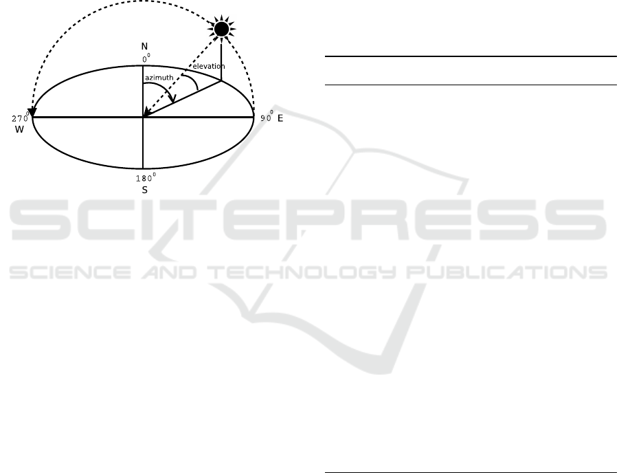
two measurements as shown in Figure 1.
Figure 1: The Sun Position Diagram.
The first measurement is the Sun’s direction on a com-
pass. A plumb line drawn from the sun to the hori-
zon intersects a specific degree on compass rows and
this angle is a measure of the Sun’s azimuth. We also
need to know Sun’s altitude or vertical angle, its an-
gular height above the horizon. The combination of
azimuth and elevation describes a specific spot on the
Skydome.
Algorithm 1 computes the sun position from sun-
rise to sunset of a specific latitude(φ) for a given
date(d) and a given interval of time in minute(τ). We
need to know two things before we calculate the Sun
position, the geographical location of the observer,
and the orientation of the Sun at that position. To de-
termine these two positions two sets of angles have to
be specified. The first set, containing two angles, pin-
points the location on earth. They are a) latitude and
b) longitude(θ). The second set of angles is related to
the position of the Sun concerning a particular loca-
tion on the earth. These angles are 1) declination an-
gle, 2) elevation/altitude angle(α), 3) zenith angle(β),
4) azimuth angle(γ), and 5) hour angle(ω). The So-
lar declination angle is the angle between the equato-
rial plane of the Earth and the rotational plane of the
Earth around the Sun explained in line 4. ∆ in line 3
is the day angle and n is the day number which varies
from 1 on January 1st to 365 (366) December 31. The
hour angle is the angular displacement of the Sun east
or west of the local meridian due to the rotation of
the Earth around its axis 15
◦
per hour; morning neg-
ative, afternoon positive and during solar noon zero.
The hour angle for sunrise (ω
sr
) and sunset (ω
ss
) is
explained in line 5 and line 6, respectively. Line 7
converts the time interval τ to angle in radian τ
ω
. The
loop at line 8 calculates the hour angles, I
ω
from sun-
rise to sunset. Line 12 calculates the elevation angle
at hour angle ω
i
. The solar azimuth angle calculated
through line 13 to 17 is the angular distance of the
Sun’s projection on the horizontal plane at a place on
earth from a reference direction. Different authors use
different conventions for calculating solar azimuth an-
gle. In this paper, the azimuth angle is measured from
the north clockwise from zero to 360
◦
.
Algorithm 1: Sun Position Calculation from Sunrise to Sun-
set.
1: procedure SUNPOS(φ, τ, d )
2: n = dayofyear(d)
3: ∆ = (2.0 × π × n)/365.25
4: δ = sin
−1
(0.3978 × sin(∆ − 1.4 + 0.0355 ×
sin(∆ − 0.0489)))
5: ω
ss
= cos
−1
(−tan(φ)× tan(δ))
6: ω
sr
= −ω
ss
7: τ
ω
= τ × 0.261799
8: for (i = ω
sr
; ω
ss
≤ ω
sr
; i = i + τ
ω
) do
9: I
ω
= i
10: end for
11: for each ω
i
∈ I
ω
do
12: α[i] = sin
−1
(sinδ × sin φ + cos δ ×
cosω
i
× cos φ)
13: γ
0
= cos
−1
(sinδ × cos φ − cos δ ×
cosω
i
× cos φ)/cosα
14: if (i
ω
≥ 0) then
15: γ
0
= 360
◦
− γ
0
16: end if
17: γ[i] = γ
0
18: i++
19: end for
20: Return α,γ
21: end procedure
2.2 Shadow Geometry
The foundation of all science and technology is math-
ematics, and one of the most important beaches of
mathematics is trigonometry. This section defines a
set of trigonometric equations for shadow length cal-
culation. These equations can be generalized to get
the shadow top co-ordinate.
In Figure 3, 4OPQ form a right angle triangle con-
sidering the fencepost OQ of height, h drove perpen-
A Novel 2.5D Shadow Calculation Algorithm for Urban Environment
275
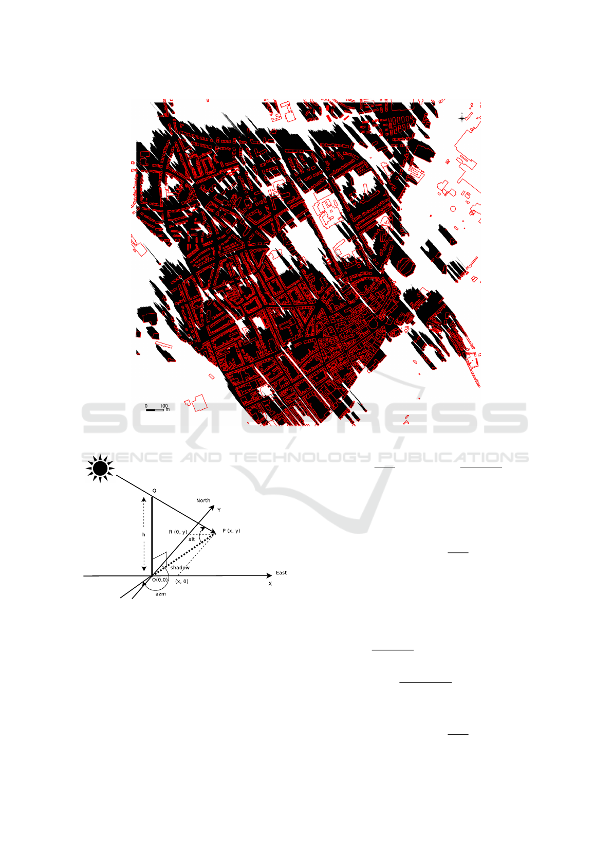
Figure 2: Date: 22nd December Time: 08:30.
Figure 3: Shadow Calculation.
dicularly into the ground. Now the question is where
would the shadow fall? However, its very easy to fig-
ure it out by drawing a line from sun across the top of
the fencepost all the way to the ground. In this case,
the length of the shadow |OP| can be calculated using
the acute angle between the horizon and the line to
the sun, alt(∠OPQ) in Equation 1. The angle alt is
commonly known as elevation angle or altitude angle.
tan(alt) =
h
| OP |
⇒ | OP | =
h
tan(alt)
meter.
(1)
The goal is to calculate the tip of the shadow lo-
cated at P(x, y), i.e. x meter East and y meter North
of the the base of the fencepost. Using right triangle
trigonometry on 4ORP, we get,
sin(azm − 180
◦
) =
x
| OP |
⇒
x = | OP | × sin(azm − 180
◦
) meter. (2)
azm is a horizontal angle measured clockwise from a
north base line, commonly known as solar azimuth
angle. Substituting |OP| from Equation 1 to Equation
2.2 yields x in Equation 3.
x =
h
tan(alt)
× sin(azm − 180
◦
)
= −
h sin(azm)
tan(alt)
meter (3)
The same way, y can be calculated by Equation 2.2
and Equation 5.
cos(azm − 180
◦
) =
y
| OP |
⇒
GISTAM 2019 - 5th International Conference on Geographical Information Systems Theory, Applications and Management
276

Figure 4: True line and its approximation.
y = | OP | × cos(azm − 180
◦
) meter (4)
y =
h
tan(alt)
× cos(azm − 180
◦
) =
−
h cos(azm)
tan(alt)
meter (5)
Therefore, from Equation 3 and Equation 5 the
shadow tip coordinate can be observed at
P =
−
h sin(azm)
tan(alt)
, −
h cos(azm)
tan(alt)
2.3 Bresenham’s Line Drawing
Algorithm
Bresenham’s line algorithm named after the inventor
Jack Elton Bresenham (Bresenham, 1965) is a funda-
mental line drawing algorithm in computer graphics.
Its primary use it to draw lines on raster graphics de-
vices. The line-drawing algorithm is based on draw-
ing an approximation of the real line, which is diffi-
cult to be drawn due to low precision caused by pixel
spacing on a PC monitor especially when dealing with
low resolutions.
In Figure 4, the true line is indicated in white
straight line starting from (0,0) to (9,6), and its ap-
proximation is indicated in black cells along the true
line. Bresenham’s line-drawing algorithm works in
the following ways; first, it decides which axis is the
major axis and which is the minor axis based on the
length. X axis is the major axis in Figure 4. Starting
from the original position, in each iteration, the cur-
rent value of the major axis is incremented by exactly
one cell (pixel). Then it decides the most appropri-
ate pixel on the minor axis for the current pixel of the
major axis by checking which pixel’s center is closer
to the true line. Bresenham’s algorithm for approxi-
mate line drawing is all about this decision making. It
is not 100% precise but works effectively for higher
resolution.
3 METHODOLOGY
The 2.5D shadow of the buildings are generated by
executing SHADOW2D, explained in Algorithm 2 and
the entire process is illustrated using a block-diagram
in Figure 5. In line 2, the building heights are obtained
by subtracting the base height of the building from the
DSM. BLDHEIGHT performs this task as illustrated in
Algorithm 3. The DSM data is derived from a LiDAR
survey which gives directly the surface model in a de-
sired resolution. To obtain the building base heights
we used a tool called 3Dfier
1
(Biljecki, 2017) which
was developed by Delft University. It takes building
footprints and a LiDAR point cloud to extrude the
footprints to a LOD1 model in which buildings are
represented by block models (usually extruded foot-
prints). The base height of the resulting building cube
is based on descriptive statistics like the height values
of the 10% quantile of the points falling inside the
footprint. With available base heights linked to each
building footprint it is then easy to compute the differ-
ence between the top of the DSM and bottom of each
building to get the building height. sunpos t gets so-
lar orientation by means of azimuth and altitude angle
for a given date and time for each and every point in
the give building footprint.
sunpos t calls SUNPOS, described in Section 2.1
with two additional parameter time and building foot-
print in line 3. The coordinates function generate
the Cartesian co-ordinates for each and every point in
the given building footprint. From north (N), south
(S), east (E) and west (W) values first, the four coor-
dinate corners, (W,S); (E,S); (E,N); (W,N) and
hence the coordinate of each and every point in the
building footprint is computed, respectively in line
4. From line 5 to 8 the algorithm is computing the
shadow tops (x
>
,y
>
) for each point (x,y) in building
footprint flowing the trigonometric formulation de-
rived in Section 2.2. Bresenham’s line drawing algo-
rithm explained in Section 2.3 is used to connect each
(x,y), (x
>
,y
>
) pair in the grid to draw the shadow line.
4 CASE STUDY
A proof of concept is developed for the validation
of technical feasibility of the proposed algorithm at
a very high spatial resolution by using scalable ten-
sor data structure and inherent parallelism offered by
data-flow based implementation in Tensorflow.
We run our proof-of-concept on Esch-sur-Alzette
(49
◦
29
0
44.988
00
N, 5
◦
58
0
50.016
00
E), located 5,505.41
1
https://github.com/tudelft3d/3dfier
A Novel 2.5D Shadow Calculation Algorithm for Urban Environment
277
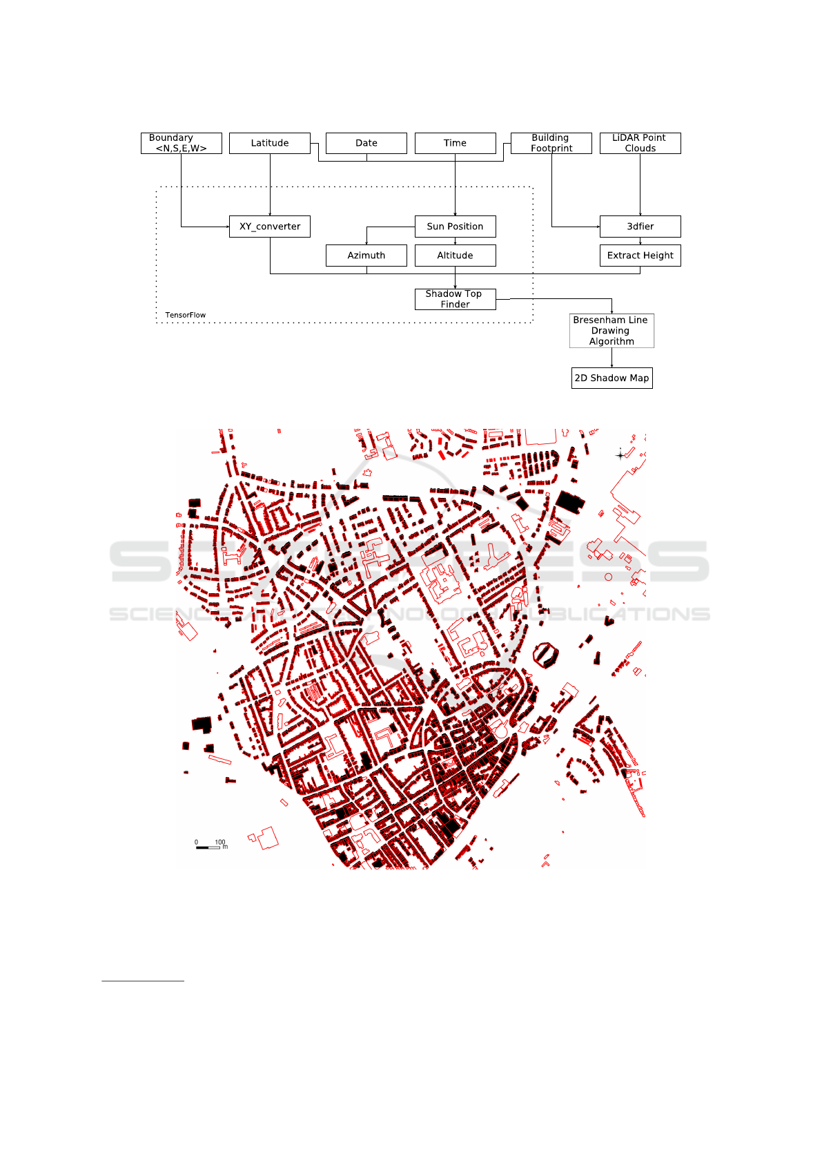
Figure 5: Block Diagram of Shadow Calculation Approach.
Figure 6: Date: 21st June December Time: 11:30.
km north of the equator, in the northern hemisphere
2
. It is situated in south-western Luxembourg on the
border with France, the second largest town after the
country’s capital Luxembourg city. The total area
2
https://fr.distance.to/Esch-sur-Alzette
of 14.35 km
2
with elevation above sea level ranging
from 279m to 426m. In this paper, we used a digital
elevation model of Esch-sur-Alzette. The grid is 1874
columns by 1828 rows, with a spatial resolution of 1
meter. The sun orientations from sunrise to sunset on
GISTAM 2019 - 5th International Conference on Geographical Information Systems Theory, Applications and Management
278
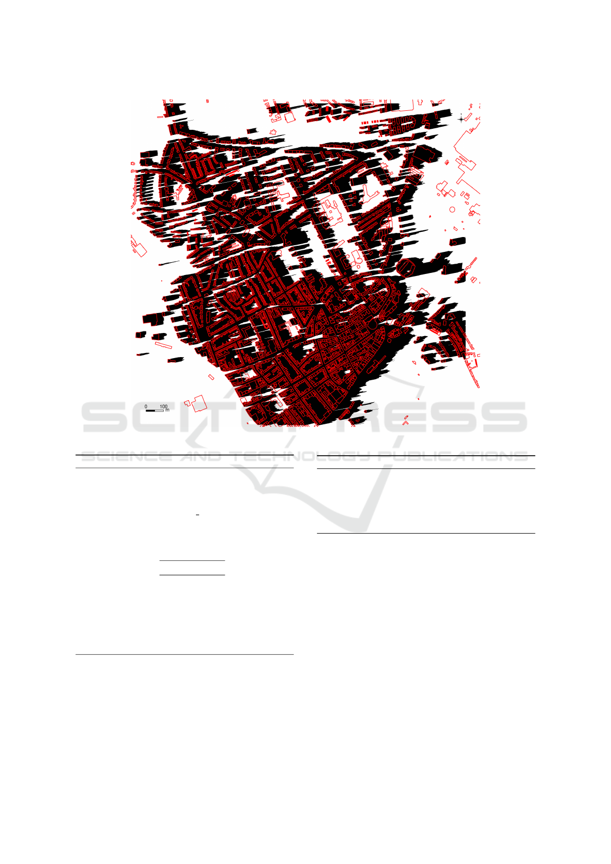
Figure 7: Date: 23rd September Time: 16:30.
Algorithm 2: 2.5D shadow calculation of buildings.
1: procedure SHADOW2.5D(hN,S,E,Wi, φ, d, t,
Bld
footpnt
, LiDAR
ptcld
)
2: H = BLDHEIGHT(Bld
footpnt
, LiDAR
ptcld
)
3: azm, alt = sunpos t(SUNPOS(φ, τ, d), t,
Bld
footpnt
)
4: XY = coordinates(hN,S,E,Wi, Bld
footpnt
)
5: for each hx,yi ∈ XY do
6: x
>
= −
H[x,y] * sin(azm)
tan(alt)
7: y
>
= −
H[x,y] * cos(azm)
tan(alt)
8: end for
9: for each hx,yi ∈ XY & each hx
>
,y
>
i ∈ XY
>
do
10: print
pixel
(bresenham(x,y,x
>
,y
>
))
11: end for
12: end procedure
21
st
June, 23
rd
September, 22
nd
March and 22
nd
December are shown in Figure 9. SUNPOS (Algorithm
1) is used to generate the result. We plotted Figures of
cast shadow simulations for some exemplary sun po-
sitions over the year, namely, 23
rd
September at 08:30
(Figure 2), 21
st
June (Figure 6) at 11:30, 22
nd
Decem-
Algorithm 3: Building height calculation.
1: procedure BLDHEIGHT(Bld
footpnt
, LiDAR
ptcld
)
2: Bld
LOD1
= 3dfier(Bld
footpnt
, LiDAR
ptcld
)
3: Bld
ht
= extract
ht
(Bld
LOD1
)
4: Return Bld
ht
5: end procedure
ber at 16:30 (Figure 7). The Figures showing building
footprints of Esch-sur-Alzette in red outlines and ar-
eas in black are covered by cast shadows of the build-
ings. The direction and length of the cast shadows are
determined by the position of the sun (Figure 2.1).
The town gets longer cast shadows when the sun po-
sition is low over the horizon in the morning (Fig-
ure 2) and evening (Figure 7) hours, and short and
more crisp shadows (Figure 6) when the sun reaches
zenith about mid day. One can clearly notice the
difference of sun position and resulting cast shadow
length and the influence to neighbouring buildings or
areas. Some unfavorable locations can end up receiv-
ing much less direct sunlight during the course over
the year due to their relative position to other objects.
A Novel 2.5D Shadow Calculation Algorithm for Urban Environment
279
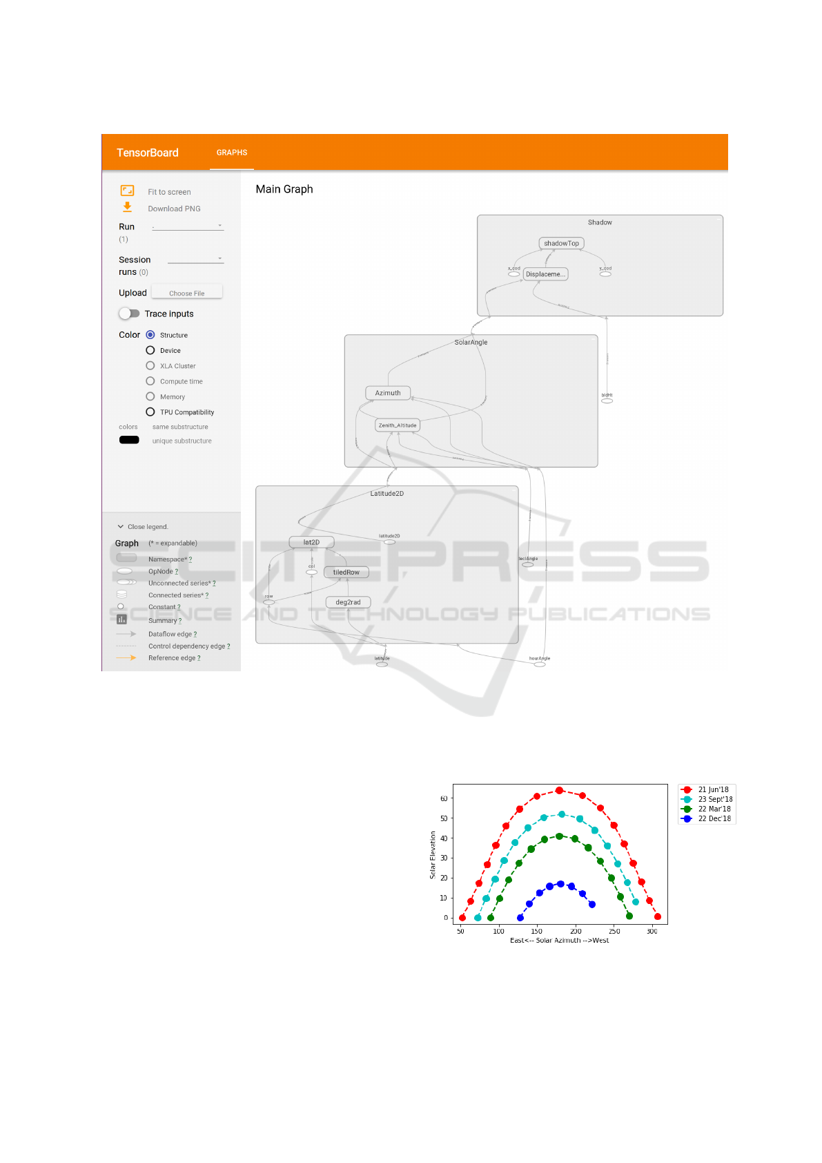
Figure 8: Dataflow graph generated by TensorBoard.
4.1 Performance
The proof of concept run on a 64 bit ma-
chine with Intel(R) Core(TM) i7-6800K CPU @
3.40GHz processor. The performance is quite sig-
nificant. Figure 2, Figure 6 and Figure 7 took
42.26 secs, 29.63 secs and 113.20 secs, re-
spectively. The performance is remarkably faster
than r.sunmask module by Geographic Resources
Analysis Support System, commonly referred to
as GRASS (GRASS Development Team, 2017).
r.sunmask Calculates cast shadow areas from sun
position and DSM if the sun position is specified or
based on given date/time calculates the sun position
by itself.
The underlying data-flow graph of the implemen-
tation of the algorithm is shown in Figure 8 using Ten-
sorboard. Tensorboard is the interface included with
any standard TensorFlow installation used to visual-
ize the data-flow graph and other tools to understand,
debug, and optimize the model.
Figure 9: Sun path for Esch-sur-Alzette Calculated using
Algorithm 1.
GISTAM 2019 - 5th International Conference on Geographical Information Systems Theory, Applications and Management
280

5 CONCLUSIONS
The main characteristics of the proposed 2.5D shadow
implementation can be described as follows,
• Defining, optimizing, and efficiently calculat-
ing mathematical expressions involving multi-
dimensional arrays (tensors).
• Transparent use of GPU computing. One can
write the same code and run it either on CPUs or
GPUs.
• Implicit parallelism and distributed execution.
• High scalability of computation across machines
with huge data sets.
The building heights are valid for flat roofs (L0D1
model). This flatness of the terrain affects the accu-
racy of the cast shadows. In our future work, we are
considering digital elevation model to get the actual
hight of the object, towards a more accurate and ro-
bust shadow map.
ACKNOWLEDGEMENTS
This work has been funded and supported by the EN-
OVOS Foundation Luxembourg and the Luxembourg
Institute of Science and Technology (LIST) through
the SECURE project.
REFERENCES
Abadi, M., Agarwal, A., Barham, P., Brevdo, E., Chen, Z.,
Citro, C., Corrado, G. S., Davis, A., Dean, J., Devin,
M., Ghemawat, S., Goodfellow, I., Harp, A., Irving,
G., Isard, M., Jia, Y., Jozefowicz, R., Kaiser, L., Kud-
lur, M., Levenberg, J., Man
´
e, D., Monga, R., Moore,
S., Murray, D., Olah, C., Schuster, M., Shlens, J.,
Steiner, B., Sutskever, I., Talwar, K., Tucker, P., Van-
houcke, V., Vasudevan, V., Vi
´
egas, F., Vinyals, O.,
Warden, P., Wattenberg, M., Wicke, M., Yu, Y., and
Zheng, X. (2015). TensorFlow: Large-scale machine
learning on heterogeneous systems. Software avail-
able from tensorflow.org.
Appel, A. (1968). Some techniques for shading machine
renderings of solids. In Proceedings of the April
30–May 2, 1968, Spring Joint Computer Conference,
AFIPS ’68 (Spring), pages 37–45, New York, NY,
USA. ACM.
Biljecki, F. (2017). Level of detail in 3D city models.
PhD thesis, Delft University of Technology, Delft, the
Netherlands.
Biljecki, F., Stoter, J. E., Ledoux, H., Zlatanova, S., and
C¸
¨
oltekin, A. (2015). Applications of 3d city models:
State of the art review. ISPRS Int. J. Geo-Information,
4(4):2842–2889.
Bresenham, J. E. (1965). Algorithm for computer control
of a digital plotter. IBM Syst. J., 4(1):25–30.
GRASS Development Team (2017). Geographic Resources
Analysis Support System (GRASS GIS) Software, Ver-
sion 7.2. Open Source Geospatial Foundation.
Whitted, T. (1980). An improved illumination model for
shaded display. Commun. ACM, 23(6):343–349.
A Novel 2.5D Shadow Calculation Algorithm for Urban Environment
281
