Phase Distribution in Probabilistic Movement Primitives, Representing
Time Variability for the Recognition and Reproduction of Human
Movements
Vittorio Lippi and Raphael Deimel
Technische Universit
¨
at Berlin, Fachgebiet Regelungssysteme, Sekretariat EN11, Einsteinufer 17, 10587 Berlin, Germany
Keywords:
ProMP, Human Movement, Prediction, Recognition, Time Warping, Phase.
Abstract:
Probabilistic Movement Primitives (ProMPs) are a widely used representation of movements for human-robot
interaction. They also facilitate the factorization of temporal and spatial structure of movements. In this work
we investigate a method to temporally align observations so that when learning ProMPs, information in the
spatial structure of the observed motion is maximized while maintaining a smooth phase velocity. We apply
the method on recordings of hand trajectories in a two-dimensional reaching task. A system for simultaneous
recognition of movement and phase is proposed and performance of movement recognition and movement
reproduction is discussed.
1 INTRODUCTION
Overview. Probabilistic movement primitives
(ProMP) (Paraschos et al., 2013) are a representation
of movements used in robot control and human-robot
interaction (HRI) applications (Maeda et al., 2017)
and provide several desirable properties to model
tasks for robot control and HRI(Paraschos et al.,
2018). One of these properties is temporal scaling:
the movement trajectory is not a direct function of
time but function of a phase variable, φ(t), i.e. the
temporal evolution of φ determines the the velocity of
the movement independently of the spatial structure.
A ProMP represents a sample movement y(t) as
y(t) =
q
˙q
= Φ(φ(t))w + ε (1)
where q is the vector of variables describing the
movement (usually joint angles or hand effector posi-
tion and orientation) and Φ is a Nx2 vector computed
with Gaussian functions and their derivatives:
Φ
i
=
e
(φ(t)−c
i
)
2
/h
i
∑
N
k=1
e
(φ(t)−c
k
)
2
/h
k
(2)
where c
i
represents the center and h
i
expresses the
spread of the bell-shaped feature. The vector w is
drawn from a multinomial distribution which is de-
fined by its parameters θ:
p(w|θ) = N (µ
w
,Σ
w
) (3)
0 0.2 0.4 0.6 0.8 1
phase
0
0.5
1
a
0 0.5 1 1.5 2 2.5 3
time [s]
0
0.5
1
phase
b
0 0.5 1 1.5 2 2.5 3
time [s]
0
0.5
1
c
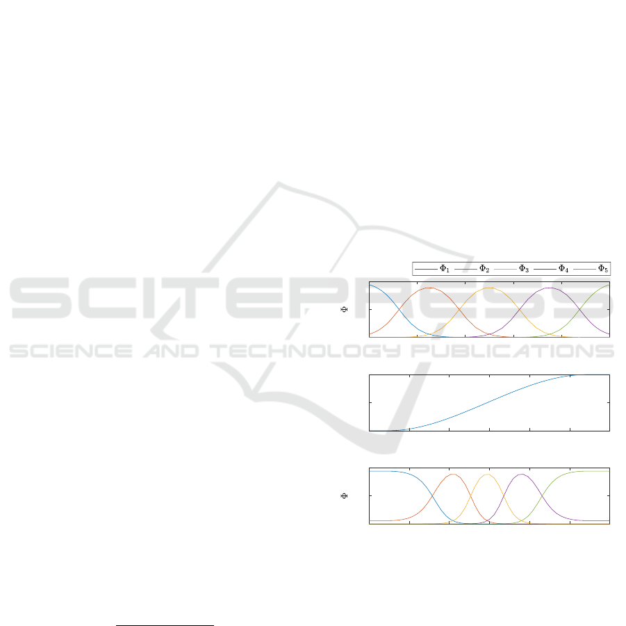
Figure 1: Features and Phase. In (a) the features Φ
i
(φ) are
represented as a function of the phase. In (b) a phase profile,
based on the beta function as a function of time. In (c) the
features are represented as a function of the time.
In a general formulation (see for example (Colom
´
e
et al., 2014)) ε in Eq. 4 models unbiased noise as
p(ε) = N (0, Σ
y
). In this paper we assume that all
the variability observed on y should be accounted by
the distribution of w and that ε ≈ 0. In this way
each observed trajectory y
i
is represented by a single
Lippi, V. and Deimel, R.
Phase Distr ibution in Probabilistic Movement Primitives, Representing Time Variability for the Recognition and Reproduction of Human Movements.
DOI: 10.5220/0007750205710578
In Proceedings of the 16th International Conference on Informatics in Control, Automation and Robotics (ICINCO 2019), pages 571-578
ISBN: 978-989-758-380-3
Copyright
c
2019 by SCITEPRESS – Science and Technology Publications, Lda. All rights reserved
571

weight vector w
i
. Vice versa, w can be interpreted as
a compressed representation of the movement trajec-
tory, obtained from projecting trajectory values onto a
lower dimensional subspace using the Moore-Penrose
pseudo-inverse of Φ:
w = Φ
+
y (4)
Which weight vector is most likely depends on the
optimization criterium, e.g. jerk minimization as reg-
ularization principle (Paraschos et al., 2018). Alter-
native features for movement representation can be
designed to guarantee other properties such as min-
imal error at the final position and speed (Lippi et al.,
2012). Due to the probabilistic nature of the ProMP
framework constrains on generated trajectories can
be imposed by conditioning the probability distribu-
tion(Paraschos et al., 2018). Figure 1 illustrates the
features as either a function of time or phase. The
time modulation performed by the phase function also
modulates the resolution of the low dimensional rep-
resentation during movement execution. In Figure
1 (c) features in the middle of the movement are more
dense than at the beginning or at the end, due to the
choice of a sigmoidal phase profile. We assume that
part of the variability observed among the repetitions
of a movement is caused by shifted and stretched
phase signals. Time scaling can be performed by
means of a linear constant, i.e. φ = αt (Maeda et al.,
2017; Ewerton et al., 2015). In this work we esti-
mate phase profile parameters for each observation
that minimize the variances over all observed w (or,
equivalently of the response in phase domain), under
the constraint of an assumed structure for the phase
profile. In particular we propose to restrict phase sig-
nals to the beta function:
φ
∆
1
,∆
2
(t) =
Z
t
0
β
2,2
τ − ∆
1
∆
1
− ∆
2
dτ (5)
where β
2,2
is the incomplete beta function with pa-
rameters a = b = 2. This sigmoidal function, shown
in 1 (b), is differentiable, monotonic and saturates at
0 and 1. The parameters ∆
1
, ∆
2
associated with each
trajectory depend on the distribution of the whole
sample set. Notice that weights w are in general spe-
cific w.r.t. to the chosen phase profile (see Eq. 4). The
average of the sample set distribution is defined as:
y = argmin
e
y
N
∑
i=1
Z
1
0
(y
i
(φ) −
e
y(φ))
2
dφ (6)
For the i
th
sample the phase is defined as:
φ
i
= argmin
e
φ
Z
1
0
y
i
e
φ(τ(φ))
− y(φ)
2
dφ (7)
The term τ(φ) represents alignment between the av-
erage y and the y
i
sample, it express the fact that as
e
φ and φ are both monotonically dependent on t, the
former can be expressed as a function of the latter, in
particular:
τ(φ) = arg
t
φ(t) =
e
φ(t)
(8)
As y depends on all phase profiles, Eq.6 and Eq.7
need to be optimized together to find the optimal
phase profiles. The problem is solved by iteratively
optimizing φ(t) and φ
i
, which yields phase profile pa-
rameters for each sample movement. The phase pro-
file parameters of the average trajectory is fixed a pri-
ori to ∆
1
= ∆
2
= 0, as the time scaling when com-
paring two or more movements (e.g. when comput-
ing the average) depends on the relationship between
the respective phase profiles and hence there is a de-
gree of redundancy. The described time scaling can
also be performed on time domain values. In order to
take into account the movement primitive representa-
tion the y in Eq. 6 and Eq. 7 can be projected on the
MP representation y
mp
= Φw. Once optimized time
scaling parameters of the sample set are obtained,
we can obtain a probability distribution describing
the movements using empirical estimators from lit-
erature (Maeda et al., 2017; Paraschos et al., 2018).
In the following paragraphs we demonstrate (a) how
to identify a model for movements, (b) how to recog-
nize an observed movement given a set of movement
primitives, (c) how to estimate the current phase, (d)
how to integrate perception in the phase recognition
process and (e) how to generate a movement.
Model Identification. The estimation of ProMP pa-
rameters from of a sample set can be based on dif-
ferent principles, e.g. linear regression of each ob-
servation individually (Paraschos et al., 2013) or
maximizing the likelihood of the complete observed
data(Paraschos et al., 2018). As introduced in the
overview in this work we assume ε ≈ 0 in Eq. 4 and
that the phase profile can be chosen to minimize the
variability on w. This leads to a two step procedure:
First, each observed trajectory is assigned a set of pa-
rameters (w
i
,∆
1i
,∆
2i
). This is done on the basis of Eq.
6 and Eq. 7 to obtain the phase profile, and Eq. 4 to
obtain w, then the distributions for w (Eq. 2) and φ(t)
is obtained with an empirical estimator. An example
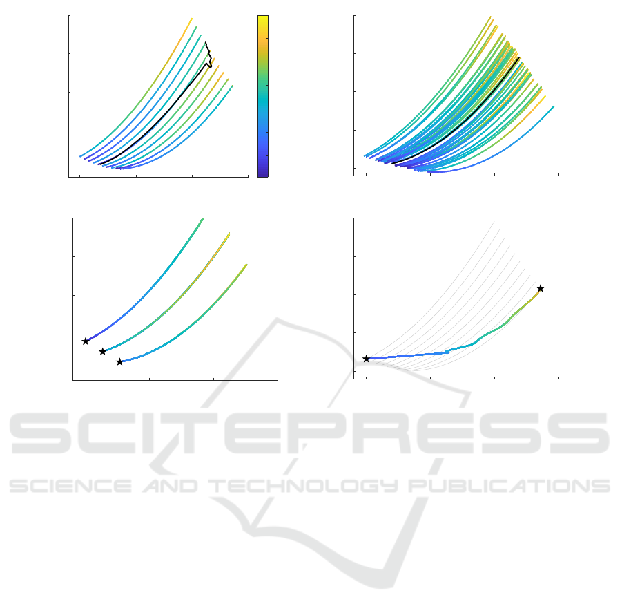
of model identification is shown in Fig.2. The train-
ing set is generated artificially and consists of planar
motion with random time profile (with the form spec-
ified in Eq.5) and non-intersecting parabolic trajecto-
ries. In Fig.2 (b) movements generated with the iden-
tified distribution are shown. Notice that assuming
a normal distribution of w produces a distribution of
trajectories that is different from the more “uniform”
training set.
ICINCO 2019 - 16th International Conference on Informatics in Control, Automation and Robotics
572

Movement Recognition. An observed movement y
can be classified by comparing likelihoods between
ProMPs. The likelihood
p(y(t
i
)|µ
k
,Σ
k
)
=
R
1
0
p
y(t
i
)|Φ(φ)µ
k
,Φ(φ)Σ
k
Φ(φ)
T
p(φ|t
i
)dφ
(9)
of observing the movement given model k is com-
puted and the most likely model is selected, i.e. L =
argmax
k
p(y|θ
k
). Notice that the probability of y(t
i
)
is considered independent of the previous observa-
tions, i.e. p(y(t
i
)|θ
k
,y(t
i−1
)) = p(y(t
i
)|θ
k
). The prob-
ability of an observed sequence can be obtained by
multiplying the probabilities of the observed samples,
p(y|θ
k
) =
∏
t
f
0
p(y
t
|θ
k
). In the described examples
we will include all the past observations of y
t
, in the
general case not all points of the trajectory may be
available, due to occlusion for example. Applying the
ProMP framework to such cases is demonstrated in
(Maeda et al., 2017).
Phase Recognition. Using the Bayes rule we can
estimate the most likely phase of an observed sample:
p(φ|y(t
i
)) =
p(y(t
i
)|Φ(φ)µ
k
,Φ(φ)Σ
k
Φ(φ)
T
)p(φ|t
i
)
∑
M
k
p(θ
k
)p(φ|y(t), θ
k
)
(10)
Notice that p(φ|t
i
) is assumed to be normally dis-
tributed and hence parameterized by mean µ
φ
(t) and
standard deviation σ
φ
(t) as functions over time. ∆
1
and ∆
2
are not normally distributed due to the nonlin-
ear relationship in Eq. 5. In most prior work on the
topic, φ is assumed to be a linear function over time
and that therefore φ(t) can be described by a normal
distribution, e.g. in (Ewerton et al., 2015). Dynamic
time warping (DTW) is another, nonlinear, approach
proposed recently (Ewerton et al., 2018).
Perception. Eq. 10 provides an estimate given a
time-dependent but otherwise fixed p(φ|t
i
) derived
from the training set. Alternatively, we can use an
explicit phase estimate provided by some perceptual
system. Examples of fusing ProMP and perception
have been proposed, e.g. in (Dermy et al., 2019)
ProMPs are used in the context of predicting human
intentions. In general the sensor input will have many
more dimensions than y. In this work we will estimate
the phase from recent observations of the motion. We
will consider a phase estimator based on previous val-
ues of y over a sliding time window to yield an esti-
mate φ
∗
(t
i
) of the current phase. Such estimator is
used to compute the probability of the observed y(t
i
).
Instead of integrating over the distribution of proba-
bility of φ as shown in Eq. 9, only the estimated value
is used to compute y(t
i
):
p(y(t
i
)|µ
k
,Σ
k
)
= p
y(t
i
)|Φ(φ
∗
(t
i
))µ
k
,Φ(φ
∗
(t
i
))Σ
k
Φ(φ
∗
(t
i
))
T
(11)
Movement Generation. The model can be used
to generate movements. Depending on the task the
movements can be generated deterministically using
Eq. 1 or stochastically by sampling w from the dis-
tribution. In certain cases the term ε in Eq. 1 may be
nonzero due to actuation and external noise, but is not
the case in the presented example. Generating move-
ments from ProMP can be used both for robot con-
trol and to predict human movements in HRI, see, for
example, (Oguz et al., 2017). Samples can obey con-
straints such as a specific target position or velocity,
by conditioning the distribution to the constraint prior
to sampling (Paraschos et al., 2013), which can be
done parameterically (and therefore efficiently) with
normal distributions. A constraint can be expressed
as a target point y
∗
(φ
i
) to be reached at a given phase.
Exploiting the linear dependency between w and y the
updated parameters for p(w|y
φ
i
= y
∗
(φ
i
)) are
µ
∗
w
= µ
w
+Σ
w
Φ
T
(φ)
Φ(φ)Σ
w
Φ
T
(φ)
−1
(y
∗
− Φ(φ)µ
w
)
(12)
Σ
∗
w
= Σ
w
+ Σ
w
Φ
T
(φ)
Φ(φ)Σ
w
Φ
T
(φ)
−1
Φ(φ)Σ
w
(13)
An example of generated movements is shown in
Fig.2 (b,c,d). The conditioned distributions in 2 (c)
exhibit very small Σ
w
(i.e. all the trajectories start-
ing from a given point are indistinguishable in shape),
capturing the regularity of the training set. In Fig.2
(d) the distribution is forced to pass through two via-
points that are unlikely to be observed in the same
movement, i.e. it is conditioned on an outlier. As
a consequence, the resulting sampled trajectories do
not resemble the observations presented in the train-
ing set.
2 DATASET AND BENCHMARK
PROBLEM
The Reaching data set consists in a reaching task:
Participants have been asked to move the mouse cur-
sor from a starting point to targets appearing in 4
different positions. Each target identifies a different
movement, associated to a different ProMP model.
The samples are shown in Fig. 3. Given the na-
ture of the task, consisting in reaching movements,
it comes natural to perform the segmentation on the
Phase Distribution in Probabilistic Movement Primitives, Representing Time Variability for the Recognition and Reproduction of Human
Movements
573
0 0.5 1 1.5
x
0
0.5
1
1.5
2
y
Training set
a
0.1
0.2
0.3
0.4
0.5
0.6
0.7
time[s]
0 0.5 1 1.5
x
0
0.5
1
1.5
2
y
Movements Generated from distribution
b
0 0.5 1 1.5
x
0
0.5
1
1.5
2
y
Conditioned distributions
c
0 0.5 1 1.5
x
0
0.5
1
1.5
2
y
Unlikely trajectory
d
Figure 2: Parabolic lines synthetic data set. In (a) an artificial data-set of trajectories with a parabolic shape and random
duration is shown, with only 10 of the 100 produced samples shown but covering more intermediate positions. The color
gradient indicates the temporal evolution of the trajectory, the black line the average trajectory in time. The resulting shape
does not match the presented examples well, especially in the end when sample count drops. The data-set has been used as a
training set for a proMP model. In (b) trajectories generated with the proMP distribution are shown, the black line represent
the average (computed respect to phase). Notice that while the model captured very accurately the shape of the movements,
the gaussian distribution of parameters results in a distribution of trajectory that is different from the one presented in the
training set. In (c) conditioned trajectories with imposed via-points a time t = 0 are shown, indicated by black stars. The
conditioned Σ
w
is so small that the trajectories generated for each via-point are indistinguishable. In (d) the trajectory is
conditioned to pass through two via-points unlikely to appear in the same movement. The resulting shape is dissimilar to
those presented in the training set. For reference, trajectories from the training set are shown in gray.
basis of events, in particular: (a) a movement starts
when the mouse cursor is in the starting position and
the target is shown on the screen and (b) it stops
when a target is reached. In general different heuris-
tics are possible for segmentation, notably the ProMP
framework provides the possibility to segment the
signal exploiting an expectation-maximization algo-
rithm, treating segmentation as a latent variable to be
optimized together with the movement models param-
eters(Lioutikov et al., 2017). The dataset includes 100
movement samples used as training-set for the model
identification and 100 samples used as test set for the
movement recognition and phase recognition. Move-
ments were sampled at 100 Hz. The number of fea-
tures was set to N = 9, with parameters, in Eq. 2,
c
k
= (k − 1)/(N − 1) and h
k
= 0.15.
3 RESULTS
Model Identification, Movement Recognition and
Phase Recognition. The distribution of phase pro-
files obtained with Eq. 6, Eq. 7 is shown in Fig 4
(b). Each sample is transformed in an MP, i.e. the pa-
rameters (w,φ) are extracted, 4 ProMP models repre-
senting the 4 movements are estimated. The observed
movement is identified as belonging to the most likely
model to produce it according to Eq. 9. The move-
ment recognition is performed at each time step. The
classification accuracy increases with time as shown
in Fig. 5 (a), and reaches 100% at the end of the
movement when movements are unambiguously dif-
ferentiated by their position. Phase recognition is also
performed for each time step using Eq. 10. The phase
estimate is obtained sample-by-sample and need not
ICINCO 2019 - 16th International Conference on Informatics in Control, Automation and Robotics
574
0 0.2 0.4 0.6 0.8 1
Horizontal Position [screen ratio]
0
0.2
0.4
0.6
0.8
1
Vertical Position [screen ratio]
a
mov 1
mov 2
mov 3
mov 4
target
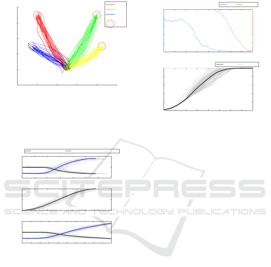
Figure 3: Reaching data set. A two-dimensional reaching
task is performed by a test participant on a computer screen
using a mouse. The participant was asked to perform the
movement as fast as possible to reach circular targets that
were appearing in a position randomly decided among 4.
The resulting set is composed by 25 repetitions of 4 distinct
targets.
0 0.1 0.2 0.3 0.4 0.5 0.6 0.7
Time [s]
0
0.5
1
position [screen ratio]
a
0 0.1 0.2 0.3 0.4 0.5 0.6 0.7
Time [s]
0
0.5
1
Phase
b
0 0.1 0.2 0.3 0.4 0.5 0.6 0.7 0.8 0.9 1
Phase
0
0.5
1
position [screen ratio]
c
Average Horizontal Trajectory Average Vertical Trajectory Samples
Figure 4: Dataset ”mov 1” (see Fig. 3). (a) shows vertical
and horizontal coordinates over time, gray lines represent
training data, black line the average. In (b) the correspond-
ing phase profiles are shown, in gray the ones associated
with the observations, in black the average one. In (c) the
resulting movements over phase are shown.
be monotonic as shown in 5 (b).
Movement Generation. In order to generate con-
crete movements the parameters w are sampled from
the distribution. Fig. 6 shows movements generated
with and without constraints. The constraint is ex-
pressed as a via-point to be reached at a given phase.
The constrained movements are generated from the
conditioned distribution with parameters from Eq. 12,
Eq. 13. In Fig. 6(a) the imposed via-point is within
the space of the presented examples and hence trajec-
0 0.1 0.2 0.3 0.4 0.5 0.6 0.7 0.8
Time [s]
0
20
40
60
80
100
Classification Error [%]
0
20
40
60
80
100
Sample Trajectories [%]
a
Error # Samples
0 0.1 0.2 0.3 0.4 0.5 0.6 0.7 0.8
Time [s]
0
0.2
0.4
0.6
0.8
1
Phase
b
Average Repetitons
Figure 5: Movement and phase recognition accuracy eval-
uated on a test set of 100 samples (25 for each of the 4
recognized movements). In (a) the relative error is shown
as a function of time (blue). As the different test samples
have different durations. The number of available move-
ment samples compared at a given time is shown (orange).
The classification error decreases from random (75%) as
more of the sample movement is observed. In (b) the es-
timated phases are shown (gray). Notice that the likelihood
of every phase value is computed at each point in time using
Eq. 10 and the most likely phase is selected. The resulting
phase signal differs from the ones assumed to generate the
training set (Eq. 5), and in general is not guaranteed to be
monotonic. Nevertheless, the average phase (black) recov-
ers the typical sigmoidal profile.
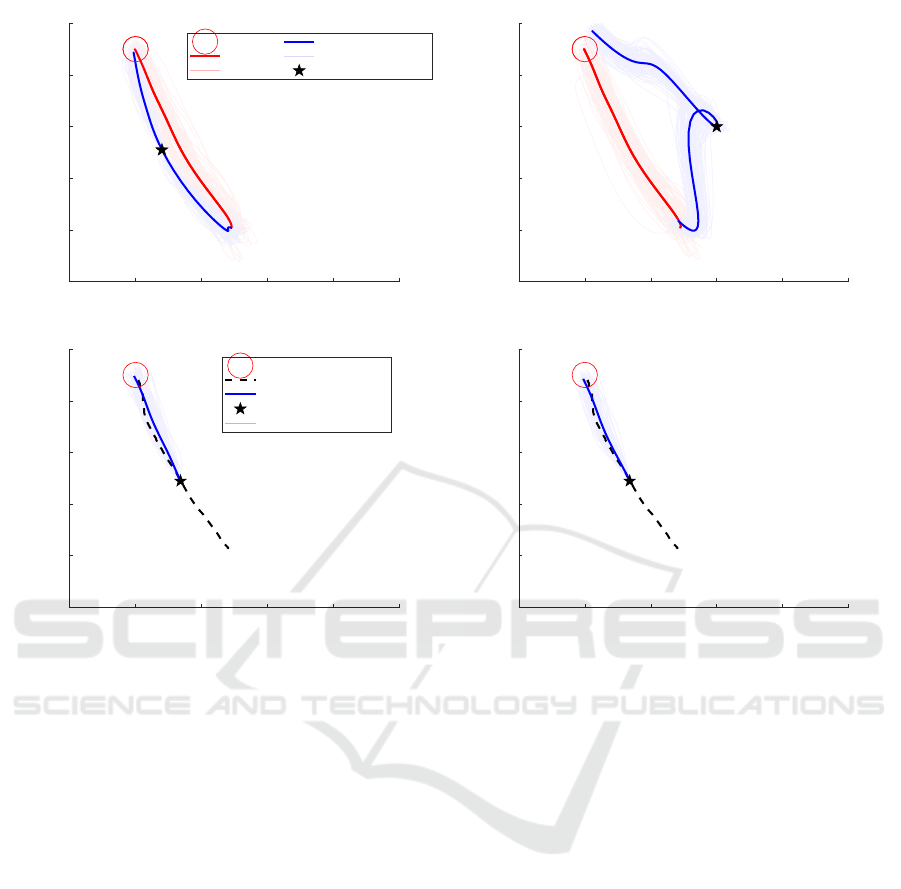
tories resemble those presented in the training set. In
Fig. 6 (b) the via-point is more distant from the posi-
tions presented in the training set and hence the condi-
tioned trajectories are less representative of the orig-
inal distribution, e.g. forming loops and missing the
final target. In (c) the conditioned distribution is used
to predict a continuation of the current motion. The
prediction is also affected by the uncertainty about the
current phase, which is estimated according to Eq. 10.
Perception. Perceptual estimation of phase was im-
plemented with a feedforward neural network with
three layers with 40, 20 and 10 neurons respectively,
taking as input the current time and a vector of 20
previous samples. The network has been trained
with the Levenberg-Marquardt backpropagation algo-
rithm(Levenberg, 1944; Marquardt, 1963). The re-
sults are shown in Fig. 7 where the classification task
(shown in Fig. 7) is repeated by exploiting the es-
timated phase, according to Eq. 11. Classification
performance using the neural network is comparable
to that obtained by integrating the phase distribution
(Eq. 9). In Fig. 6 (d) the phase estimated by the neural
Phase Distribution in Probabilistic Movement Primitives, Representing Time Variability for the Recognition and Reproduction of Human
Movements
575
0 0.2 0.4 0.6 0.8 1
Horizontal Position [screen ratio]
0
0.2
0.4
0.6
0.8
1
Vertical Position [screen ratio]
Movement from MU e sigma
a
Target
Average
Repetitions
Conditioned Average
Conditioned repetitions
Conditioned Waypoint
0 0.2 0.4 0.6 0.8 1
Horizontal Position [screen ratio]
0
0.2
0.4
0.6
0.8
1
Vertical Position [screen ratio]
b
0 0.2 0.4 0.6 0.8 1
Horizontal Position [screen ratio]
0
0.2
0.4
0.6
0.8
1
Vertical Position [screen ratio]
Prediction
c
Target
Observed Movement
Predicted
Position at Prediction Time
Conditioned repetitions
0 0.2 0.4 0.6 0.8 1
Horizontal Position [screen ratio]
0
0.2
0.4
0.6
0.8
1
Vertical Position [screen ratio]
d
Figure 6: Movements generated using the ProMP model for the observations set ”mov 1” (see Fig. 3). Trajectories in red
are samples from the distribution over w. Trajectories in blue are samples constrained to pass through a via-point at phase
φ
∗
= 0.5, indicated by a black star. Thick lines indicate the average trajectories of the respective distributions. The red circle
marks the final target. In (a) the via-point is within the space of the presented examples and hence the trajectories resemble
thoses presented in the training set. In (b) the via-point is an outlier to the positions presented in the training set and hence the
conditioned trajectories are not representative of the observed movements. In (c) the conditioned distribution is used together
with classification and phase identification to produce a prediction of the motion in progress (black dotted line). The most
likely trajectory is plotted with the blue thick line, and samples as thin blue lines. In (d) the prediction is performed using a
neural network to estimate the phase.
network is used to perform a prediction on the basis
of the observed trajectory. The result is similar to that
which is shown in Fig. 6 (c).
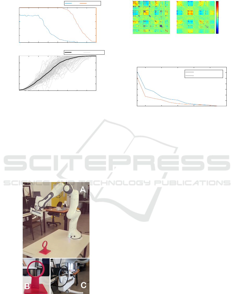
A 7-DoF Robot Arm Example. In additon to previ-
ous low-dimensional examples, model identification
is applied to movements of a 7-DoF robotic arm.
The task consists in picking up an object using a
hook and handing it to an user in a single continuous
movement. The setup is shown in Fig. 8. The ob-
ject’s loop represents a spatial constraint for the tra-
jectory, since the object is always picked up in the
same position. Trajectory examples were recorded by
manually moving the robot, producing a total of 11
examples. The task was represented in seven dimen-
sional joint space. The number of features was set to
9, hence the ProMP distribution has 63 dimensions.
Fig. 9. shows the covariance matrices of the ProMP’s
distributions learned on data without and with opti-
mized phase profiles. The use of phase modulation
decreases variation in adjacent feature weights in the
covariance matrix elements as temporal noise is ex-
ternalized to the phase signal. A more compact de-
scription of the concept is shown in Fig. 10, where
the eigenvalues of the two covariance matrices, i.e.
the principal components, are compared. All the non-
zero eigenvalues are smaller with phase modulation.
4 DISCUSSION AND FUTURE
WORK
In this work we used ProMPs to model human move-
ments and demonstrations to robots in order to per-
ICINCO 2019 - 16th International Conference on Informatics in Control, Automation and Robotics
576
0 0.1 0.2 0.3 0.4 0.5 0.6 0.7 0.8
Time [s]
0
20
40
60
80
100
Classification Error [%]
0
20
40
60
80
100
Sample Trajectories [%]
a
Error # Samples
0 0.1 0.2 0.3 0.4 0.5 0.6 0.7 0.8
Time [s]
0
0.2
0.4
0.6
0.8
1
Phase
b
Average Repetitons
Figure 7: Classification and phase evaluation accuracy us-
ing a neural network for the identification of phase. The
training set and the test set are the same as used in Fig. 5.
In (a) the relative error is shown as a function of time (blue).
As the movements have different durations, the number of
available movement samples at a given time is indicated
in orange. The classification accuracy increases as more
of the test movements are observed. In (b) the identified
phase profiles are shown in gray, where phase is computed
at each time step. The average phase (black) shows the typ-
ical sigmoidal profile. Although in some cases the phase
appears less accurate using the neural network estimator,
overall classification performance is comparable to that of
Fig. 5.
Figure 8: The robot task configuration (A). The robot’s
gripper is holding a hook (B) which it uses to pick up the
object (C).
form movement recognition and movement genera-
tion, with particular emphasis on leveraging a para-
-0.3
-0.2
-0.1
0
0.1
0.2
-0.2
0
0.2
Figure 9: Color representation of the covariance matrix for
w, for the robot arm movements set without phase modula-
tion (left) and with phase scaling (right). Most of the values
in the covariance matrix are smaller.
2 4 6 8 10 12
Eigenvalue #
0
0.5
1
1.5
2
2.5
3
3.5
Var
With Phase scaling
Without Phase scaling
Figure 10: Non-zero eigenvalues of the covariance matrices
shown in Fig. 9. With the phase modulation all eigenvalues
are smaller, which indicates a more precise reproduction of
movements.
metric phase profile to modulate movement execution
speed. The approach showed to properly classify and
generalize the movements in a data-set of reaching
movements. The proposed parametric phase profile
has a sigmoidal shape that is particularly suitable to
reaching tasks such as the one presented into the ex-
ample and other ”real world” tasks, such as pick and
place operations where it is relevant to the control of
initial and final position. However, a sigmoidal phase
profile enforces zero velocity at the beginning and at
the end of the movement. Therefore, in tasks where
final velocity must be controlled, other profiles (e.g.
a beta function with a = 2, b = 1) may be favorable.
In general it should be considered that time scaling of
human movements can work differently depending on
the task and the working conditions(Zhang and Chaf-
fin, 1999). The example reaching task is represented
as a library of 4 ProMPs describing movements to 4
possible targets. In general, the diversity of move-
ments in a task can be represented with a manifold in
the space of hyper-parameters and mixture distribu-
tions (Rueckert et al., 2015), or specifically with gaus-
sian mixtures describing the distribution of w (Ewer-
ton et al., 2015). The parameters can be constrained
with linear relationships for dimensionality reduction,
as recently shown in (Colom
´
e and Torras, 2018). With
human movements, dependencies between target po-
sitions and the moving parameters can be represented
by a linear model(Avizzano and Lippi, 2011; Lippi
et al., 2012). In all those cases phase can be estimated
online while observing the movement by modifying
Phase Distribution in Probabilistic Movement Primitives, Representing Time Variability for the Recognition and Reproduction of Human
Movements
577

Eq. 10 to take into account the chosen distribution.
Further, a specific perceptual estimator dedicated to
the identification of phase using a feed-forward neu-
ral network was described and implemented. The es-
timator led to a performance in terms of classification
and prediction accuracy that was comparable to that
of the system exploiting the empirical probability dis-
tribution of the phase directly. An advantage of us-
ing a neural network is, that it avoids the potentially
costly computation of the integral in Eq.9 at each inte-
gration step. Future work on phase recognition will be
focus on the identification of state of dynamic system
models tasked with generating phases, e.g. phase-
state machine models (Deimel, 2019). Such mod-
els could provide phase profiles and could be used
in conjunction with a library of ProMPs to control a
task. Furthermore, current research on ProMPs in-
cludes the design of feedback control systems consid-
ering physical interaction with the environment and
the users (Paraschos et al., 2018; Paraschos et al.,
2013). Time scaling does not apply to the control of
arm kinematics and the external contact forces in the
same way as for movements (this holds for each kind
of rescaling, also the linear one). A general frame-
work that can scale kinematics and contact instants in
time should be integrated with a consistent control of
applied forces and torques.
ACKNOWLEDGEMENTS
We gratefully acknowledge financial support for the
project MTI-engAge (16SV7109) by BMBF.
REFERENCES
Avizzano, C. A. and Lippi, V. (2011). A regression model
for digital representation of juggling. In BIO Web of
Conferences, volume 1, page 00006. EDP Sciences.
Colom
´
e, A., Neumann, G., Peters, J., and Torras, C. (2014).
Dimensionality reduction for probabilistic movement
primitives. In Humanoid Robots (Humanoids), 2014
14th IEEE-RAS International Conference on, pages
794–800. IEEE.
Colom
´
e, A. and Torras, C. (2018). Dimensionality reduc-
tion in learning gaussian mixture models of move-
ment primitives for contextualized action selection
and adaptation. IEEE Robotics and Automation Let-
ters, 3(4):3922–3929.
Deimel, R. (2019). A dynamical system for governing con-
tinuous, sequential and reactive behaviors. In Pro-
ceedings of the Austrian Robotics Workshop, page (in
press).
Dermy, O., Charpillet, F., and Ivaldi, S. (2019). Multi-
modal intention prediction with probabilistic move-
ment primitives. In Human Friendly Robotics, pages
181–196. Springer.
Ewerton, M., Neumann, G., Lioutikov, R., Amor, H. B.,
Peters, J., and Maeda, G. (2015). Modeling spatio-
temporal variability in human-robot interaction with
probabilistic movement primitives. In Workshop on
Machine Learning for Social Robotics, ICRA.
Ewerton, M., Rother, D., Weimar, J., Kollegger, G.,
Wiemeyer, J., Peters, J., and Maeda, G. (2018). As-
sisting movement training and execution with visual
and haptic feedback. Frontiers in neurorobotics,
12:24.
Levenberg, K. (1944). A method for the solution of cer-
tain non-linear problems in least squares. Quarterly
of applied mathematics, 2(2):164–168.
Lioutikov, R., Neumann, G., Maeda, G., and Peters,
J. (2017). Learning movement primitive libraries
through probabilistic segmentation. The International
Journal of Robotics Research, 36(8):879–894.
Lippi, V., Avizzano, C. A., and Ruffaldi, E. (2012). A
method for digital representation of human move-
ments. In RO-MAN, 2012 IEEE, pages 404–410.
IEEE.
Maeda, G. J., Neumann, G., Ewerton, M., Lioutikov,
R., Kroemer, O., and Peters, J. (2017). Probabilis-
tic movement primitives for coordination of multi-
ple human–robot collaborative tasks. Autonomous
Robots, 41(3):593–612.
Marquardt, D. W. (1963). An algorithm for least-squares
estimation of nonlinear parameters. Journal of
the society for Industrial and Applied Mathematics,
11(2):431–441.
Oguz, O. S., Sari, O. C., Dinh, K. H., and Wollherr, D.
(2017). Progressive stochastic motion planning for
human-robot interaction. In Robot and Human In-
teractive Communication (RO-MAN), 2017 26th IEEE
International Symposium on, pages 1194–1201. IEEE.
Paraschos, A., Daniel, C., Peters, J., and Neumann, G.
(2018). Using probabilistic movement primitives in
robotics. Autonomous Robots, 42(3):529–551.
Paraschos, A., Daniel, C., Peters, J. R., and Neumann,
G. (2013). Probabilistic movement primitives. In
Advances in neural information processing systems,
pages 2616–2624.
Rueckert, E., Mundo, J., Paraschos, A., Peters, J., and Neu-
mann, G. (2015). Extracting low-dimensional control
variables for movement primitives. In Robotics and
Automation (ICRA), 2015 IEEE International Confer-
ence on, pages 1511–1518. IEEE.
Zhang, X. and Chaffin, D. B. (1999). The effects of
speed variation on joint kinematics during multiseg-
ment reaching movements. human movement science,
18(6):741–757.
ICINCO 2019 - 16th International Conference on Informatics in Control, Automation and Robotics
578
