
Homography and Image Processing Techniques for Cadastre Object
Extraction
Lemonia Ragia
1
and Froso Sarri
2
1
School of Architecture, Technical University of Crete, Campus Kounoupidiana, 73100 Chania, Crete, Greece
2
School of Electronic and Computer Engineering, Technical University of Crete,
Campus Kounoupidiana, 73100 Chania, Crete, Greece
Keywords: Close-range Photogrammetry, Cadaster, Image Analysis, Object Extraction.
Abstract: In this paper we propose a simple, low-cost, fast and acceptable method of surveying which contributes to the
cost reduction of the service and makes it affordable for all citizens. The approach described in this paper
results in taking semi-automatically the geometry of a spatial object in a parcel for cadastre purposes, namely
swimming pool. The most innovative part of this approach is that we extract the geometry from images using
an uncalibrated camera. Normally for professional tasks we use metric or stereo cameras. The approach is
focused on simplicity and automation and little intervention of the user is required. It takes into account
images taken with an uncalibrated digital camera and cadastral spatial data. The camera is like an input device
for spatial data acquisition. Digital images acquired by a non-professional camera are usually taken by a
person, without any specific knowledge for the images or usage of the cameras. The basic concept is that the
owner of a parcel can update the data of his property by himself. The data are imported at the cadastre maps
it the end.
1 INTRODUCTION
The methods used today for carrying out a cadastral
survey rely mainly on classical survey tools and
photogrammetry. These include Electro optical
Distance Measurement Equipment (EDM), the
Global Navigation Satellite Systems (GNSS) and
Total Stations. The results of such measurements
have to comply with high accuracy. Photogrammetric
methods have been applied to cadastral surveying in
the last decades.
Modern photogrammetric techniques have been
proved to be as accurately as the classical surveying
methods. Photogrammetry uses metric cameras that
means elements of the internal orientation are known.
These include the image coordinates of the principal
point, the focal length of the camera, the fiducial
marks and the lens distortion. Photogrammetric
techniques for cadastral was first introduced in
Switzerland (Weissmann, 1971). Aerial photography
has been used for the identification of land parcels
(Siriba, 2009) then the parcel boundaries are
identified and scaled off the orthophotographs
monoscopically, and therefore sufficient for cadastral
purposes (Konecny, 2008). The identification of land
parcel boundaries using digital photogrammetric
method can be extracted by on Digital
Photogrammetric Workstation (DPW) (Kyutae and
Song, 2011). Unmanned Aerial Vehicles have been
used for cadastral mapping extracting line features
from images [UAV] (Crommelinck et al., 2016).
In our approach we try to obtain accurate
information about land from interpretation and
measurements taken from images. The images are
obtained from amateur, uncalibrated cameras.
Amateur cameras have been used since 1990s and this
approach was either single image analysis or bundle
block adjustment for relative orientation and the
creation of stereo models. Extracting a spatial object
from images taken from an uncalibrated camera is
inherently ambiguous and not trivial. The algorithms
developed require no knowledge of the camera’s
internal parameters (focal length, aspect ratio,
principal point) or external ones (position and
orientation). We use only some scene constraints such
as planarity of points, parallelism of lines and
perpendicularity of lines. The geometric constraints
are derived directly from the images due to special
markers. A hierarchy of the algorithms to calculate
points measurements is investigated and different
Ragia, L. and Sarri, F.
Homography and Image Processing Techniques for Cadastre Object Extraction.
DOI: 10.5220/0007772203050310
In Proceedings of the 5th International Conference on Geographical Information Systems Theory, Applications and Management (GISTAM 2019), pages 305-310
ISBN: 978-989-758-371-1
Copyright
c
2019 by SCITEPRESS – Science and Technology Publications, Lda. All rights reserved
305

cases are taken into account. This leads to extremely
flexible method which can be applied to different
images. In order to achieve the goal of this project, a
number of research areas had to be addressed. The
main idea was to extract the outer contour of the
house with interesting outlines, and the contour of the
swimming pool. This method has been used to update
the cadastre maps from any user and it is mainly
concerned to identify each user’s own new spatial
object, mainly swimming pool, in the cadastre map
and not to survey it with high accuracy.
Our framework is based on the principals of single
or multiview geometry, which is the concept of
acquiring metric information from a perspective view
of a scene given only minimal geometric information
determined from the image (Criminisi et al., 2000).
The method provides us with data from a simple
image, without prior knowledge of the camera
parameters (intrinsic parameters), its exact position
and free of camera synchronization or calibration.
The implemented techniques aim to increase the level
of automation, making the framework as free of user
input as possible and independent of special
equipment.
In a typical photogrammetric process stereo
vision has been used to compute depth, but, in our
case monocular vision proves to be sufficient.
2 PROPOSED METHODOLOGY
Our goal is to create a service for any user with a high
level of automation. We want to keep the user
interaction at the minimum and have the smallest
amount of photographic input. The approach
presented here uses single image analysis and
involves the steps segmentation, clustering, and edge
detection to minimize the user intervention.
Images are characterized by perspective distortion
which refers to the transformation of objects by
appearing significantly different than in the real life
form. This is due to the angle of view of the image
capturing. Shape is distorted in perspective imaging.
Parallel lines can look as if they meet in images and
rectangles appear as quadrilaterals. In order to obtain
accurate geometric information of the real world
space via an image, it is mandatory to eliminate the
perspective distortion. To that aim we need to create
a relation between the image and the real scene
depicted. Such relations often refer to the existence of
a known shape, which is in our approach a rectangle,
in the real world which is used as a reference on the
image. By knowing an area on the image which in real
life represents a rectangle, can help us make the
required association to correct the distortion. Having
considered the above, we need to create a rectangle
on the scene, which will be included on the image.
2.1 Homography
The connection of real world data with their image
representations or how the scenes depicted in images
correspond to the real world are topics that concern a
wide range of scientific fields, from computer vision
to topography. The digital depiction of the real world
has its base on perspective geometry. The distortion
that physical scenes have in images is represented in
perspective transformation. Perspective
transformation maps points to points or lines to lines
in different spaces with often non equal dimensions.
This transformation is known as homography. Given
an image of a planar surface, points on the image
plane can be mapped into corresponding points in the
world plane by means of homography (Hartley and
Zisserman, 2000). The relation between real world
and image points is
X = Hx
(1)
where x is an image point and X is the corresponding
point in real world (Criminisi, 2002). This relation is
defined by the 3x3 matrix H. The matrix H holds the
information of the transformation and therefore can
relate any image point to its position on the physical
space.
As it has become clear the main problem is the
estimation of the homography matrix H. There is a
variety of algorithms developed for estimating the H
matrix e.g. RANSAC. They are categorized based on
three methods for acquiring H, using
nonhomogeneous linear solution, homogeneous
solution, non-linear geometric solution (Criminisi et
al., 1999).
In our case we used a linear solution. The method
for computing H is based on the Direct Linear
Transformation (DLT) algorithm which solves a set
of variables from a set of similarity relations such as
x=Ay where A contains the unknowns. The algorithm
implemented is described by Hartley & Zisserman in
(Hartley and Zisserman, 2000), which is a normalized
DTL for 2D homographies. In order for these
algorithms to work for uncalibrated cameras, the
estimation of the homography can be achieved
directly from a set of known image-world
correspondences, such as points. The homography
transformation is described as
(2)
GISTAM 2019 - 5th International Conference on Geographical Information Systems Theory, Applications and Management
306

(3)
where
,
(4)
x', y' are the image coordinates, x, y are the real word
coordinates and H
11
, H
12
, H
13
, H
21
, H
22
, H
23
, H
31
, H
32
,
H
33
the unknown parameters. There are eight degrees
of freedom for that transformation. This means that
for four different pairs of corresponding (x', y') and
(x, y) points, we obtain a system of eight equations
which leads to the unique determination of the
transformation of all the points.
The algorithm solves the problem which is stated
as
Given n ≥ 4 2D to 2D point correspondences {
}, determine the 2D homography matrix H such
that
= H
.
There is a need of 4 known points (markers) with
real coordinates system. We found out that not every
combination of 4 points on the ground can solve the
above problem. The four points can create any
geometrical shape in the reality and this problem must
be tackled. We have tried many different geometrical
shapes in the reality and we finalize that only a
rectangle results in the best solution. The algorithm
also applies normalization of the initial data which
makes the technique independent of scale choices,
coordinate origin choices or changes. This provides
also results with higher accuracy.
The corners of a rectangle are going to be used as
the four correspondences required to compute the
homography transformation. This is a method to
create the four pairs of image to world points, while
fulfilling the requirement for perspective correction.
2.2 Automatic Swimming Pool
Extraction
2.2.1 Color based Segmentation
The identification of the pool on the image is crucial
in order to obtain information about its location. The
position of the corner pixels can be extracted if the
system can recognize the pool. Image segmentation
techniques are achieving that aim. The property that
distinguishes the pool from its neighboring
environment is its color, therefore the image is
analyzed with color-based segmentation (Cheng et
al., 2001). By performing color based segmentation,
the image is partitioned in chromatically
homogeneous regions. Each identified region has
pixels with the same chromatic values. For this
purpose, our framework used the K-means clustering
algorithm for image content classification.
2.2.2 K-means Clustering
K-means Clustering in digital imaging is a region
formation technique which relies on common patterns
in specific values within a group of neighboring
pixels (Sharma et al., 2012). Clustering distinguishes
and classifies samples with similar properties (Phyo
et al., 2015). Color based clustering creates clusters,
each one consisting of pixels with similar chromatic
properties and the goal of the segmentation algorithm
is to create clusters according to their color
homogeneity. Given an image this method splits it
into K clusters. The number of clusters (k) is decided
beforehand. Each cluster is defined by its center.
Every point is associated to the cluster where the
difference between the point and the center is
smallest. The mean is considered the center of each
cluster. After an initial assignment of all the data
points, the new means of the clusters are recalculated
and the data are reassigned to the new clusters. This
iterative process is finished when no new changes
occur in the cluster means. The objective of the
algorithm is defined as:
argmin
(5)
where
is a cluster and
is its mean.
2.2.3 Clustering Implementation
In order to chromatically segment the image, it was
transformed in the CIE L*a*b* color space. This
color space approximates the human vision. It
includes all perceivable colors and its coverage
exceeds those of other models, such as the RGB color
model. The L*a*b* space consists of a luminosity
channel L* and the color channels a* and b*. Channel
a* indicates where color falls along the red green axis,
and blue yellow colors are represented along the b*
axis. The color information is on the a* and b*
channels. Each image point is regarded as a point in
the L*a*b* color space and the difference between
two colors can be calculated as the Euclidean distance
between two color points (SCIMS 2019). The ability
to express color difference as Euclidean distance is of
great importance in color segmentation.
After converting the image in the L*a*b* color
space the k-means clustering algorithm is
implemented with 3 initial mean values. The pixels
are assigned in clusters according to their a* and b*
values. The result are three clusters, each with similar
Homography and Image Processing Techniques for Cadastre Object Extraction
307
color values. We are interested in the cluster
containing the blue objects in the image. It is
determined that the blue cluster has the smallest mean
a* and b* values, making this a criterion to
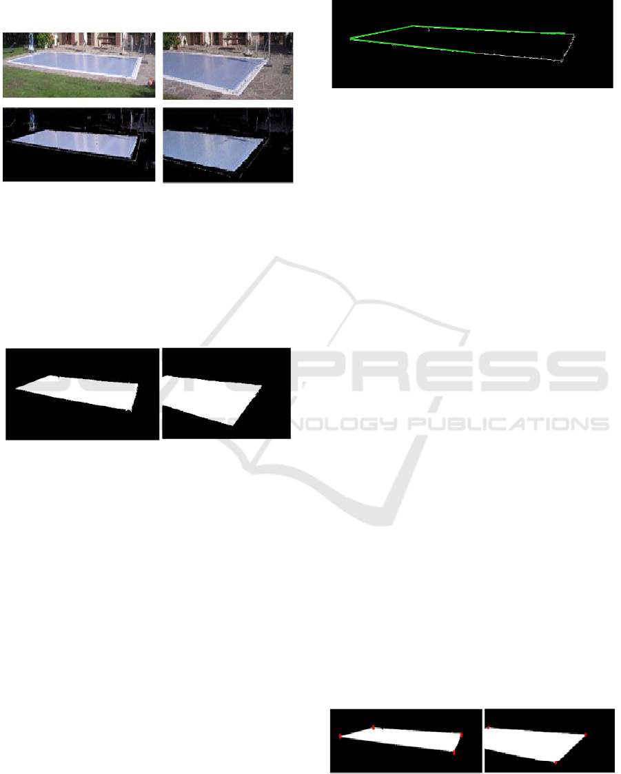
distinguish the cluster (Figure 1).
Figure 1: Input images and the identified blue cluster.
Further processing is required to define the pool.
After removing the small objects from the image, we
identified all the connected image components. It is
observed that the pool is always the biggest
component, thus removing all the other components
we refined the result which depicts only the pool in a
binary black-white image (Figure 2).
Figure 2: Final feature extraction, the pool is identified.
2.3 Corner Points Detection
Detecting corners of a quadrilateral or a rectangle in
a binary image, is a common process and a variety of
solutions are provided. There is a variety of
algorithms for that purpose, such as the Harris –
Stephens corner detector algorithm (Harris and
Stephens 1998) or the FAST algorithm (Rosten and
Drummond 2005). However, these algorithms work
better with perfectly shaped features consisting of
straight lines. Our cases involve rectangles formed by
edges with irregularities, as it is expected in images
depicting outdoor scenes. Our initial approach was
based on the Hough transform (Kovesi, 2019), which
is a feature extraction technique used to identify lines,
circles or curves. Its characteristic is that it can find
imperfect instances of those features and perform a
robust detection under noise. Hough transform
detects lines based on their polar form. Our aim was
identifying the meeting points of lines as corners after
line detection. Unfortunately even that robust
approach was unsuccessful in our cases due to the line
imperfection (Figure 3).
Figure 3: The Hough transform implemented on one of our
cases. The lines are not identified in the parts with
irregularities
Considering the unsuitability of the known
algorithms for our case, we implemented a different
method for identifying the corners. Using the binary
image from the pool extraction method, we scan the
image for the outmost occurrences of the points
belonging to the swimming pool. In this part of the
framework the input is a binary image with zeros
everywhere except the section of the swimming pool
which is represented with pixel value 1. The image is
scanned in order to find the first and last occurrences
of non zero elements belonging to the swimming
pool, in the vertical and horizontal direction. Those
are considered corners. More specifically, the image
is scanned vertically returning the row and column
pixel position of all the occurrences of the non zero
elements. The pixel position of the first and last of
those occurrences are the leftmost and rightmost
corners.
Then we single out the first and last row which
have occurrences of the non zero elements. We
identify all the non zero elements that belong in those
two rows and we sort them by their pixel values
separately in two arrays, one representing the non
zero occurrences of the first row and the other those
of the last row. The pixel position of the first element
in the first row array is the uppermost corner and the
pixel position of the last element of the last row array
is the lowermost corner. The method considerers
special cases, such as rectangles or shapes with
horizontal or vertical lines which is a rare occurrence
in images due to the perspective distortion and
recognizes the real corner points from the side points
where the swimming pool is cut out of the image
(Figure 4).
Figure 4: The identification of the corners.
GISTAM 2019 - 5th International Conference on Geographical Information Systems Theory, Applications and Management
308
2.4 Georeferencing
The resulting pixel positions of the previous step are
computed with the homography matrix and the
geographic coordinates are calculated. Our aim is to
calculate the geographic coordinates of all four
swimming pool corners. There are several approaches
to achieve that. An image with all swimming pool
corners visible along with the aforementioned
rectangle for the perspective correction can be put as
input in the framework and have immediate results.
Another approach is the input in the framework of an
image with three corners visible. The fourth corner
can be calculated via Euclidian geometry. One other
method involves the use of two images one with the
correction rectangle and one with all the corners of
the swimming pool. The two pictures can be related
with a homography matrix, essentially computing the
final geographic coordinates via a proxy image. All
three approaches were implemented.
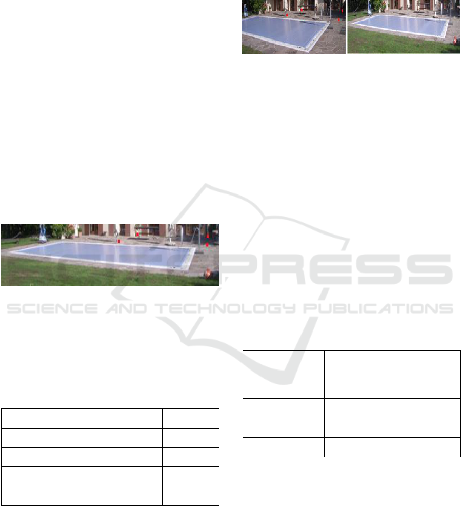
Approach A: Image with Four Visible Swimming
Pool Corners
Figure 5: Image with four swimming pool corners visible
as input.
This straight forward approach uses one image to
identify both the perspective correction rectangle
formed by the red dots on the image and the four
swimming pool corners (e.g. Figure 5). This
technique is the least accurate. The results are
presented below.
Real Geographic
coordinates
Results
Error (distance
in m)
2490643.605,
1114391.994
2490643.254,
1114391.621
0.513
2490636.025,
1114399.984
2490636.336,
1114399.791
0.366
2490632.345,
1114396.534
2490632.993,
1114397.344
1.037
2490639.925,
1114388.524
2490639.917,
1114388.631
0.108
It can be observed that the points further from the
perspective correction rectangle (e.g the third
coordinate above which represents the leftmost
corner in the image) are those with the biggest
deviation from the real coordinates. It was determined
experimentally that as we move further from the
rectangle the accuracy of the results diminishes.
Approach B: Two Images
Figure 6: Two images as input. The corners are calculated
based on the second image, whereas the perspective
correction rectangle is acquired from the first image.
The geographic coordinates in this method are
calculated from the second image using as a proxy for
the perspective correction the first image (e.g. Figure
6). In order to minimize the deviation of the results
from the first approach, the input for the initial
rectangle and the four points to be computed were
separated in two images. To be more specific, the
image which has the closest depiction of the initial
rectangle, in our case the first image above is used to
calculate the homography matrix relating the image
with the geographic coordinates. The points to be
computed are extracted from the second image which
depicts all four corners. A second homography matrix
is computed based on four random point pairs in the
two images. This matrix relates the two images. In
summation, the points are extracted from the second
image, they are transformed in the coordinate system
of the first image via the homography matrix relating
the two images and then the geographic coordinates
are computed via initial homography matrix.
Real Geographic
coordinates
Results
Error
(distance in
m)
2490643.605,
1114391.994
2490643.136,
1114391.425
0.737
2490636.025,
1114399.984
2490636.035,
1114399.393
0.592
2490632.345,
1114396.534
2490632.379,
1114397.022
0.489
2490639.925,
1114388.524
2490639.780,
1114388.351
0.225
The overall accuracy of the results is improved in
comparison to the previous method. There is a
definite rectification of the third coordinate, but a loss
in accuracy of the others. This may be due to the
errors in the point pair selection, the extra step which
involves external input.
Homography and Image Processing Techniques for Cadastre Object Extraction
309

3 CONCLUSIONS
This paper presented a simple, low-cost and fast
technique of acquiring metric information via the use
of images. This method has the potential to substitute
classic methods of surveying, in the sense that results
in obtaining geometric information at minimum cost.
It extracts information from images using an
uncalibrated camera. Utilizing the principals of single
or multiview geometry, we are provided with data
without prior knowledge of the camera intrinsic
parameters, position or orientation and free of camera
synchronization or calibration.
The algorithms developed detect automatically
the geometry of an object and compute spatial data
with the requirement of minimum scenes constraints
and user input. The principals of homography were
utilized to relate image information with geographic
coordinates. Image segmentation techniques and
morphological image processing were combined to
achieve the required automation in geometric data
extraction. Depending on the combination of the
algorithms and the variation of input, three methods
were presented to compute the final geographic
coordinates. The framework created is considered a
flexible, automatic and accurate way of acquiring
spatial data with no use of special equipment.
However, the flexibility of the framework can be
further increased by developing the methodology to
include detection of random shape spatial objects.
As further work we would like to fully automate
the approach, the user hasn’t to do any intervention.
We envision an open, interoperable application
environment for spatial information processing,
empowering the user and providing the cadastre
office with new services. The services are fed with
spatial information input, which comes from the
uncalibrated digital cameras , as well as from the
cadastre data. We are currently investigating more
algorithms and technologies for extracting spatial
information form the images independent of the
geometry of the spatial object.
ACKNOWLEDGEMENTS
This work is supported by the project Citigeo
(Citizen-centered Photogrammetry Service Project
www.citigeo.ch). We would like to thank especially
Laurent Niggeler and Geoffrey Cornette from Etat de
Genève, Prof. Dimitri Konstantas and Vedran Vlajki
Switzerland for their support.
REFERENCES
Weissmann, K., 1971. Photogrammetry Applied to
Cadastral Survey in Switzerland. Photogrammetric
Record, Vol. 7(37), 5 -15.
Siriba, D., 2009. Positional Accuracy Assessment of a
Cadastral Dataset based on the Knowledge of the
Process Steps used. Proceedings of the 12th AGILE
Conference on GIScience.
Konecny, G., 2008. Economic considerations for
phototogrammetric mapping. International Archives of
the Photogrammetry, Remote Sensing and Spatial
Information Sciences. Vol. XXXVII, part 6a. 207 – 211.
Kyutae, A., Song Y., 2011. Digital Photogrammetry for
Land Registration in Developing Countries. FIG
Working Week: Bridging the Gap Between Cultures.
Crommelinck, S., Bennett, R., Gerke, M., Nex, F., Yang,
M. Y., & Vosselman, G., 2016. Review of automatic
feature extraction from high-resolution optical sensor
data for UAV-based cadastral mapping. Remote
Sensing, 8(8). http://doi.org/10.3390/rs8080689
Criminisi, A., Reid, I., & Zisserman, A. 2000. Single view
metrology. International Journal of Computer Vision,
40(2), 123-148.
Hartley, R. I., and Zisserman, A., 2000. Multiple View
Geometry in Computer Vision. Cambridge University
Press, ISBN: 0521623049.
Criminisi, A. (2002). Single-view metrology: Algorithms
and applications. Pattern Recognition. Springer Berlin
Heidelberg, 224-239.
Criminisi, A., Reid I., and Zisserman, A., 1999. A plane
measuring device. Image and Vision Computing 17.8:
625-634.
Cheng, H. D., Jiang, X. H., Sun, Y., & Wang, J. (2001).
Color image segmentation: advances and prospects.
Pattern Recognition, 34(12), 2259-2281.
Sharma, N., Mishra, M., & Shrivastava, M. (2012). Colour
image segmentation techniques and issues: an
approach. International Journal of Scientific &
Technology Research, 1(4), 9-12.
Phyo, T. Z., Khaing, A. S., & Tun, H. M. (2015).
Classification of Cluster Area Forsatellite Image.
International Journal of Scientific & Technology
Research Volume 4, Issue 06, 393- 397.
SCIMS 2019 (Survey Control Information Management
System) http://spatialservices.finance.nsw.gov.au/
surveying/scims_online (accessed on February 2019)
Harris, C., and Stephens, M. (1998). A Combined Corner
and Edge Detector. Proceedings of the 4th Alvey Vision
Conference, 147-151.
Rosten, E., and Drummond, T. (October 2005). Fusing
Points and Lines for High Performance Tracking.
Proceedings of the IEEE International Conference on
Computer Vision, Vol. 2: 1508–1511.
Kovesi, P., 2019 MATLAB and Octave Functions for
Computer Vision and Image Processing.
Available from: http://www.peterkovesi.com/
matlabfns/. (accessed on February 2019).
GISTAM 2019 - 5th International Conference on Geographical Information Systems Theory, Applications and Management
310
