Dynamic Modeling and Simulation of a Slurry Mixing and Pumping
Process: An Industrial Case
Ridouane Oulhiq
1,2
, Khalid Benjelloun
1
, Maarouf Saad
3
, Yassine Kali
3
and Laurent Deshayes
2
1
AII Laboratory, Ecole Mohammadia d’Ing
´
enieurs, Mohammed V University, Rabat, Morocco
2
Innovation Lab for Operations, Mohammed VI Polytechnic University, Benguerir, Morocco
3
Electrical Engineering Department,
´
Ecole de Technologie Sup
´
erieure, Montreal, QC H3C 1K3, Canada
Keywords:
Mixing Tank, Centrifugal Pump, Slurry, Modeling, Simulation, Density Variation, Level Variation.
Abstract:
In this paper, a dynamic model of a slurry mixing and pumping process is proposed. The centrifugal pump
is modeled based on the hydraulic application, the hydraulic part and the induction motor models, taking into
account the pumped slurry density. This paper also proposes a new approach to estimate the parameters of the
pump’s hydraulic part model based on the pump characteristic curves. Additionally, a dynamic simulation of
the system is realized under MATLAB/Simulink environment and the variation effect of the process inputs on
the outputs is studied.
1 INTRODUCTION
In many process industries, the mixing and pumping
process is a decisive step. It is common to blend dif-
ferent products together to form a mixed slurry for
downstream processes. Eventually, the quality of the
final product will be derived by how good the mix
is and the precision of the inlet flows (Nienow et al.,
1997). Considering the widespread of such a pro-
cess, understanding its dynamics is of great impor-
tance. A steady state approach is often used to de-
scribe the system. However, a steady state process
requires constant properties. For slurry processes,
solids’ properties such as the granulometry change
as a function of time and place as does the solids’
density (Miedema, 1996). Since inlet density impacts
how easily the slurry is pumped (Blevins and Nixon,
2010), this change in density impacts the flow rate of
the slurry. Therefore, a dynamic model is needed, for
a better understanding, simulation and control of the
system.
A mathematical model, based on first order non-
linear differential equations, is used to describe the
mixing process (Deng, 2002). For the slurry pumping
process, the centrifugal pump is used. In (Kallesøe
et al., 2006), the dynamic model of the centrifugal
pump is divided into three sub parts: the pump mo-
tor, the hydraulic part and the hydraulic application.
The parameters of hydraulic part are calculated based
on the physical properties of the pump. The hydraulic
application is not detailed and the variation of flow is
not discussed. In (Valtr, 2017), the centrifugal pump
is modeled based on the hydraulic system without
considering the pump’s motor. In (Miedema, 1996) a
dynamic model for the system pump/pipeline is pro-
posed and simulated. However, the model assumes
that the pump drive behaves like a constant torque
system. Concerning the pump’s motor, the induction
motor is used. The model of the induction motor is
extensively described in literature. The most popular
representation is the so-called qd model based on a
series of mathematical transformations (Manekar and
Bodkhe, 2013). The idea of a revolving reference
frame, dq, is introduced to transform the ac compo-
nents of the vectors in the stator frame into dc sig-
nals in order to simplify calculations (Trzynadlowski,
2000).
In this work, a graphical method is used to es-
timate the pump’s hydraulic part, the head and the
load torque parameters. In literature, a numerical
method is used to calculate these parameters based on
the physical properties of the pump (Isermann, 2007;
Kallesøe et al., 2006), which is time consuming and
hard to apply in an industrial environment. For the
hydraulic application, it depends on the studied sys-
tem. A generalized method is presented in this work,
taking into account the friction factor variation along
with the slurry flow rate variation.
Oulhiq, R., Benjelloun, K., Saad, M., Kali, Y. and Deshayes, L.
Dynamic Modeling and Simulation of a Slurry Mixing and Pumping Process: An Industrial Case.
DOI: 10.5220/0007774000270035
In Proceedings of the 9th International Conference on Simulation and Modeling Methodologies, Technologies and Applications (SIMULTECH 2019), pages 27-35
ISBN: 978-989-758-381-0
Copyright
c
 2019 by SCITEPRESS – Science and Technology Publications, Lda. All rights reserved
27

The outline of this paper is as follows. Section 2
exposes the process description and dynamic analysis
of the mixing tank and the centrifugal pump. Section
3 presents the simulation and the performance results.
Section 4 concludes the paper.
2 PROCESS DESCRIPTION AND
DYNAMICS ANALYSIS
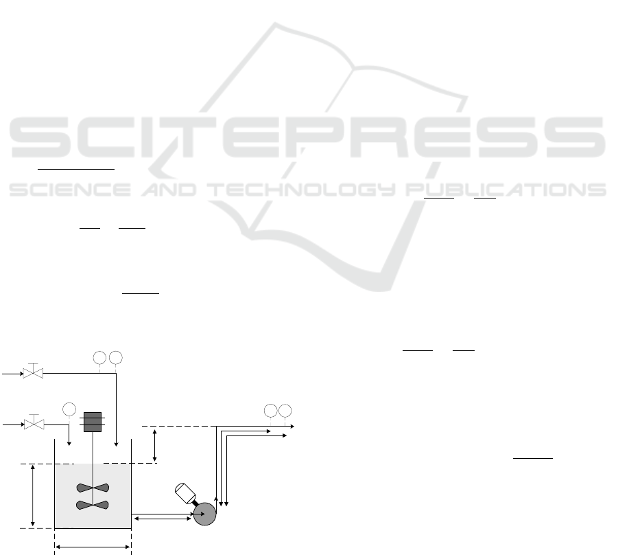
The process studied is a part of an industrial thick-
ening unit as shown in Fig. 1. The slurry arriving to
the unit is delivered to a cylindrical mixing tank in
which it is kept in agitation in order to avoid the de-
cantation of the solid. The process water is used to
adjust the solid rate of the slurry. The mixed slurry is
then pumped, using a centrifugal pump driven by an
induction motor, to downstream processes.
2.1 Dynamic Analysis of the Mixing
Tank
The dynamic behavior of the mixing tank is described
by the following equations (Skogestad, 2008; Hougen
et al., 1954):
• Conservation of the total mass in the mixing tank
d(M
pm
+ M
wm
)
dt
= d
w
F
w
+d
ps1
F
ps1
− d
ps2
F
ps2
(1)
• Level of the mixing tank:
dL
m
dt
=
4
π.D
2
m
(F
ps1
+ F
w
− F
ps2
) (2)
• Density of the slurry at the outlet of the mixing
tank:
d
ps2
=
4
πD
2
m
L
m
(M
pm
+ M
wm
) (3)
Slurry
Process water
Centrifugal pump
Mixing tank
p1
p2
Lmp
LpF
Kpt
Kmp
z2
z1
Hs
Mixed Slurry
Lm
Dm
DIT FIT
{ Fps1, dps1 }
Fw
{ Fps2, dps2 }
LpD
FIT
DITFIT
Figure 1: Pump hydraulic application parameters.
Where M
pm
is the total mass of dry product in the
mixing tank (Kg), d
ps1
is the density of slurry at the
inlet of the mixing tank (Kg/m
3
), F
ps1
is the volumet-
ric flow rate of slurry at the inlet of the mixing tank
(m
3
/s), d
ps2
is the density of slurry at the outlet of the
mixing tank (Kg/m
3
), F
ps2
is the volumetric flow rate
of slurry at the outlet of the mixing tank (m
3
/s), M
wm
is the total mass of water in the mixing tank (Kg), d
w
is the density of water (Kg/m
3
), F
w
is volumetric flow
rate of water at the inlet of the mixing tank (m
3
/s), L
m
is the level of slurry in the mixing tank (m) and D
m
is the diameter of the mixing tank (m). In what fol-
lows, it is assumed that the mixing tank is perfectly
mixed. The perfect mixing assumption is valid for
low-viscosity liquids that receive an adequate degree
of agitation (Seborg et al., 2010).
2.2 Dynamic Analysis of the Centrifugal
Pump
The flow of a centrifugal pump is related to two pa-
rameters, namely, the pump head and the system head.
The intersection of the two head curves is the flow
operating point of the system (Bachus and Custodio,
2003). The equation describing this fact is given by
the different parts of the pump.
First of all, applying Newton’s second law of mo-
tion to the fluid in the pipe (Matko et al., 2001; Valtr,
2017) yields to:
dF
ps2
dt
=
gA
p
L
mt
∆H (4)
where ∆H is the head variation (m), A
p
is the pipe
section (m
2
), L
mt
is the length of the pipe between the
mixing tank and the downstream process (m) and g is
the gravity (m/s
2
).
Then, based on (4), the equation describing the
variation of flow in function of the pump head H
p
and
the system head H
sys
is obtained:
dF
ps2
dt
=
gA
p
L
mt
(H
p
− H
sys
) (5)
2.2.1 The Hydraulic Application
The system head between p1 and p2 (Fig. 1) (Menon,
2004) is:
H
sys
= H
s
+ H
l
+ H
v
+
P
2
− P
1
d
ps2
g
(6)
where H
sys
is the system head between p1 and p2 (m),
H
s
is the static head of the system (m), H
l
is the to-
tal head losses in the system (m), H
v
is the velocity
head (m), P
1
and P
2
represent the pressure at p1 and
p2 respectively (Pa) and d
ps2
is the density of slurry
(kg/m3) (Fig. 1) with:
SIMULTECH 2019 - 9th International Conference on Simulation and Modeling Methodologies, Technologies and Applications
28

• P
1
= P
2
= P
atm
(Atmospheric pressure);
• H
v
=
v
2
2
−v
2
1
2g
;
• H
s
= z
2
− z
1
.
v
1
and v
2
are respectively the velocity at p1 and p2
(m/s) where:
• v
1
≈ 0;
• v
2
=
4F
ps2
πD
2
p
;
For the total head losses:
H
l
= H
l f riction
+ H
llocal
(7)
where H
l f riction
is the friction losses (Pa) and H
llocal
is the local losses (Pa).
The friction losses are described by the Darcy
equation (Green and Perry, 1997):
H
l f riction
=
f v
2
2
L
mt
2gD
p
(8)
Then:
H
l f riction
=
f L
mt
2gD
p
4F
ps2
πD
2
p
!
2
(9)
where D
p
is the pipe diameter (m) and f is the Darcy
friction factor.
The Darcy friction factor depends on the pipe
properties and on the nature of the pumped fluid
(Menon, 2004; El-Emam et al., 2003).
Moreover, for the local losses :
H
llocal
=
1
g
v
2
2
n
∑
i
K
i
(10)
where K
i
are are the local loss coefficients.
Then:
H
llocal
=
1
g
(K
mp
+ K
pt
)
4F
ps2
πD
2
p
!
2
(11)
where K
mp
is the local loss coefficient caused by the
sudden contraction between the mixing tank and the
pipe and K
pt
is the local loss coefficient caused by the
change in pipe geometry between the pump and the
thickener.
After simplifying (6), the relation of the system
head is obtained:
H
sys
= α + βF
2
ps2
+ γ f F
2
ps2
(12)
where :
α = z
2
− L
m
β =
1
2g

4
π.D
2
p

2
[1 + 2(K
mp
+ K
pt
)]
γ =
1
2g

4
π.D
2
p

2
L
mt
D
p
In classic pumping systems design, the friction
factor f is fixed at the beginning according to the flow
operating point (Wright and Gerhart, 2009; Chiasson,
2016). However, the friction factor depends on the
fluid velocity and properties. Thus, the friction factor
changes as the flow changes and it must be updated in
each iteration of the dynamic model simulation.
2.2.2 The Hydraulic Part
The pump head H
p
(m) is a function of flow F
ps2
and
shaft speed w
p
(rad/s). The equation describing this
fact is (Kallesøe et al., 2006; Kallesøe et al., 2004):
H
p
= a
h
F
2
ps2
+ b
h
F
ps2
.ω
p
+ c
h
ω
2
p
(13)
where a
h
, b
h
and c
h
are constant parameters fixed
from the physical properties of the pump.
However, obtaining these physical properties of
the pump is time consuming and maybe impossible
in an industrial environment. In this work, these pa-
rameters are determined using the H-Q curves of the
used pump.
The pump torque (or the load torque) T
p
(N.m)
is described by the equation (Kallesøe et al., 2006;
Kallesøe et al., 2004):
T
p
= −d
ps2
a
t
F
2
ps2
+ d
ps2
b
t
F
ps2
ω
p
+ c
t
ω
2
p
(14)
where a
t
, b
t
and c
t
are constants found from the phys-
ical properties of the pump.
In this work, these parameters are determined us-
ing the H-Q curves of the used pump.
2.2.3 The Induction Motor
The equation describing the mechanical part of the
pump is (Chan and Shi, 2011; Trzynadlowski, 2000):
dω
p
dt
=
1
J
m
+ J
p
(T
e
− T
p
) −
C
f
J
m
+ J
p
ω
p
(15)
where J
m
is the moment of inertia of the pump me-
chanical parts (Kg m
2
), J
p
is the moment of inertia
of the fluid inside the pump impeller (Kg m
2
), C
f
is
the friction losses coefficient of pump induction mo-
tor (Kg m
2
/s) and T
e
is the torque produced by the
pump induction motor (Nm).
The torque T
e
is calculated based on the electro-
mechanical and the electrical parts of the induction
motor (Chan and Shi, 2011; Trzynadlowski, 2000).
2.3 Mixing and Pumping Unit Global
Model
From the process parts dynamic analysis, the overall
model of the system is described by Fig. 2 and the
Dynamic Modeling and Simulation of a Slurry Mixing and Pumping Process: An Industrial Case
29

equations:
dL
m
dt
=
4
πD
2
m
(F
ps1
+ F
w
− F
ps2
) (16)
d(d
ps2
)
dt
=
4
πD
2
m
L
m

(d
w
− d
ps2
)F
w
+ (d
ps1
− d
ps2
)F
ps1

(17)
dF
ps2
dt
=
gA
p
L
mt

(a
h
− β − γ f )F
2
ps2
+ b
h
ω
p
F
ps2
+ c
h
ω
2
p
− α

(18)
dω
p
dt
=
1
J
m
+ J
p
(T
e
+ d
ps2
a
t
F
2
ps2
− d
ps2
b
t
F
ps2
ω
p
− c
t
ω
2
p
)
−
C
f
J
m
+ J
p
ω
p
(19)
Mixing tank
+
Centrifugal Pump
(18), (19), (20), (21)
Slurry flow rate
Fps1
Water flow rate
Fw
Slurry flow rate
Fps2
Mixing tank level
Lm
Slurry density
dps1
Slurry density
dps2
Induction motor speed
wp
Figure 2: The mixing unit bloc diagram.
The model takes into consideration the density
and the friction factor variations and assume that the
mixing tank is perfectly mixed.
The model inputs and outputs shown in Fig. 2
are as follows: The model manipulated inputs are
the slurry flow rate (F
ps1
) and the water flow rate
(F
w
); The model disturbance input is the slurry den-
sity (d
ps1
); The model outputs are the mixing tank
level (L
m
), the slurry density (d
ps2
), the slurry flow
rate (F
ps2
) and the induction motor speed (w
p
).
3 SIMULATION
3.1 Simulation Parameters
The simulation parameters are given in Table 1.
Where p is the pole number of the pump induction
motor, L
mn
is the mutual inductance of the pump in-
duction motor (H), L
s
and L
r
are the stator and the
rotor inductances (H), R
s
and R
r
are the stator and
the rotor resistances (Ω), E is The voltage of the
power supply (V), θ is the Initial phase angle of the
power supply (rad), ω is the supply angular frequency
(rad/s) and R
i
is the internal resistance of the power
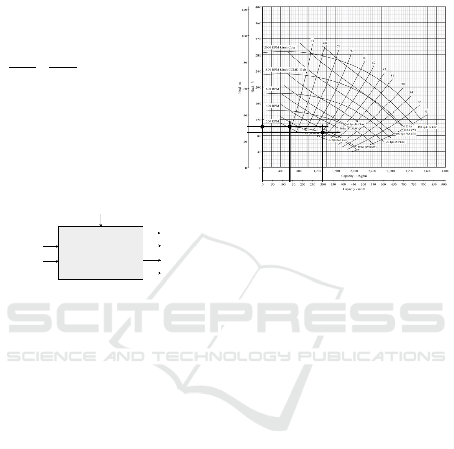
supply (Ω). To determine the parameters a
h
, b
h
and c
h
in (13), the pump characteristic curve is used. Three
different operating points are chosen (Fig. 3) in order
Figure 3: The method used to determine a
p
, b
p
and c
p
.
to get three equations with the three variables. The
solution of the system gives :



a
h
= −1.04 × 10
−4
b
h
= 1.21 × 10
−6
c
h
= 2.15 × 10
−5
(20)
To fix the parameters a
t
, b
t
and c
t
in (14), equation
(21) is used (Isermann, 2007) :
P
p
= ω
p
T
p
(21)
where P
p
is the power required by the pump.
The characteristic curve of P
p
is given in the H-
Q curve of the pump. Using this characteristic, three
different points are chosen (Fig. 4). Each point is as-
sociated with a shaft speed, flow and power. Then,
using (21), the torque T
p
is determined for each cou-
ple (shaft speed, flow). Based on (14), three equations
with the variables a
t
, b
t
and c
t
, are obtained. The so-
lution of the system gives :



a
t
= −20.23
b
t
= −1.56 × 10
−4
c
t
= 7.98 × 10
−3
(22)
3.2 Simulation Results
The simulation is done using the Matlab/Simulink
software. The simulation blocks are created based
on Level-2 Matlab s-functions. After the simulation
of the different blocks of the process, the simulation
of the whole process is done as depicted in Fig. 5.
The chosen initial parameters are: Mixing tank slurry
density : 1600 Kg/m
3
; Mixing tank level : 6 m; In-
let slurry flow rate : 300 m
3
/h; Inlet slurry density :
1600 Kg/m
3
; Inlet water flow rate : 0 m
3
/h
SIMULTECH 2019 - 9th International Conference on Simulation and Modeling Methodologies, Technologies and Applications
30

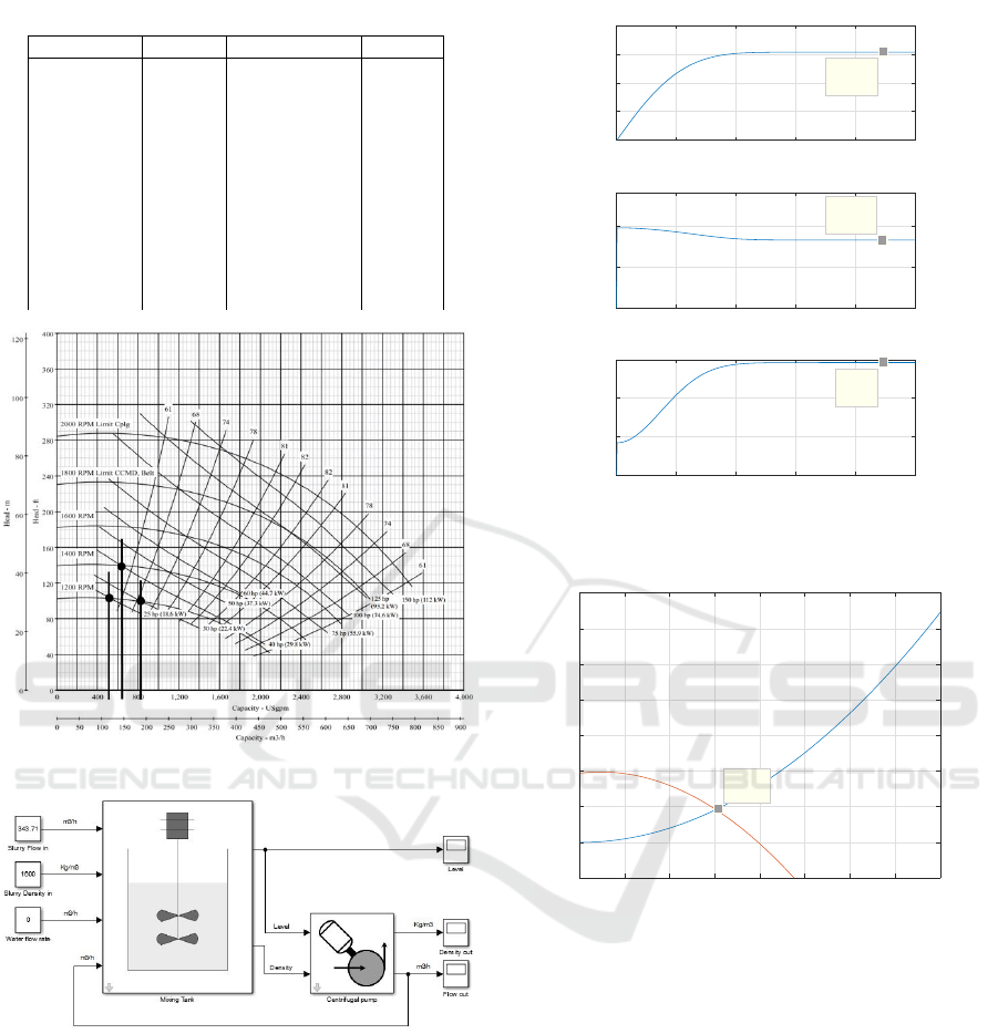
Table 1: Simulation parameters.
Parameter Value Parameter Value
D
m
(m) 13 D
p
(m) 0.4
L
mt
(m) 21 K
mp
0.5
K
pt
0.3 g (m/s
2
) 9.81
ν (m
2
/s) 0.015 ε (m) 0.07
z
2
(m) 11 J
m
(Kgm
2
) 0.4
J
p
(Kgm
2
) 0.4 C
f
(Kgm
2
/s) 0.062
p 6 L
mn
(m) 0.041
L
s
(H) 0.0425 L
r
(H) 0.0418
R
s
(Ω) 0.288 R
r
(Ω) 0.158
E (V) 220 θ (rad) 0
ω (rad/s) 2π×50 R
i
(Ω) 0.05
Figure 4: The method used to determine a
t
, b
t
and c
t
.
Figure 5: The mixing and pumping unit simulation using
Matlab/Simulink.
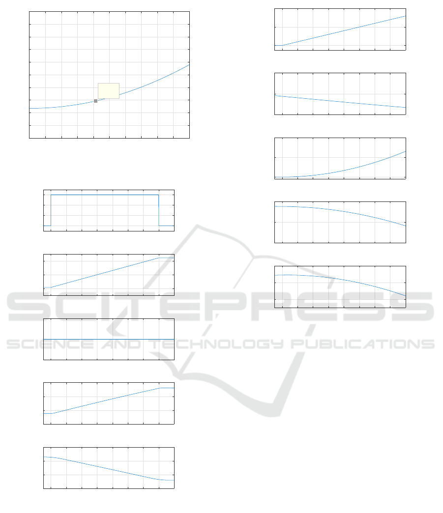
3.2.1 The System Operating Point
After the simulation is launched, the outlet flow of
the pump stabilizes at 306 m
3
/h, the induction motor
speed stabilizes at 826 rpm and the load torque at 293
Nm (6). In order to validate the operating point of
the system, the pump and the system head curves are
plotted (Fig. 7). The intersection of the two curves
gives the same flow operating point 285 m
3
/h. Then
the pump load torque is plotted in function of the in-
duction motor speed for a flow of 306 m
3
/h (Fig. 8) .
0 50 100 150 200 250
Time (s)
0
100
200
300
400
Flow (m3/h)
Outlet slurry flow rate
0 50 100 150 200 250
Time (s)
0
500
1000
Speed (rpm)
Motor speed
0 50 100 150 200 250
Time (s)
0
100
200
300
Torque (N.m)
Pump load torque
X: 223
Y: 306.8
X: 223
Y: 826.4
X: 223
Y: 293
Figure 6: The operation point of the system.
0 100 200 300 400 500 600 700 800
Flow (m3/h)
0
5
10
15
20
25
30
35
40
Head (m)
H-Q curve of the system
X: 306
Y: 9.705
Figure 7: The H-Q curve of the system.
For a speed of 826 rpm the curve gives the same load
torque 293 Nm.
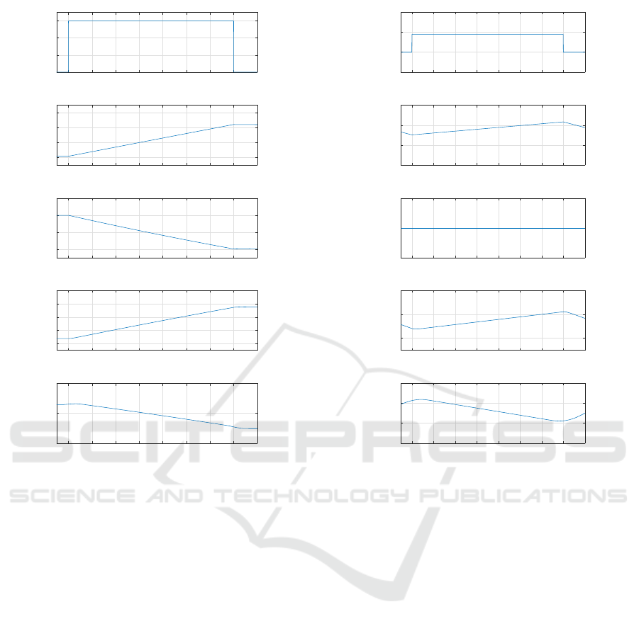
3.2.2 The System Response to Large Variations
Effect of Inlet Slurry Flow Rate Large Variation.
Keeping the inlet slurry density and the water flow
rate constants, the inlet slurry flow rate is varied. Fig.
9 shows the effect of the inlet slurry flow rate large
variation on the outputs. An increase in the inlet
slurry flow rate results in an increase in the mixing
tank level. Which results in an increase in the out-
let slurry flow rate and a decrease in the motor speed.
This is explained by a change in the static head of the
system along with a change in the load torque of the
pump.
Dynamic Modeling and Simulation of a Slurry Mixing and Pumping Process: An Industrial Case
31

0 200 400 600 800 1000 1200 1400 1600 1800 2000
Speed (rpm)
0
100
200
300
400
500
600
700
800
900
1000
Torque (N.m)
The load torque in fuction of motor speed
X: 826.8
Y: 292.5
Figure 8: The Load torque in function of motor speed.
300 400 500 600 700 800 900 1000 1100
Time (s)
300
400
500
600
Flow (m3/h)
Inlet slurry flow rate (Fps1)
300 400 500 600 700 800 900 1000 1100
Time (s)
6
6.2
6.4
Level (m)
Mixing tank level (Lm)
300 400 500 600 700 800 900 1000 1100
Time (s)
1590
1600
1610
Density (Kg/m3)
Outlet slurry density (dps2)
300 400 500 600 700 800 900 1000 1100
Time (s)
306
307
308
309
Flow (m3/h)
Outlet slurry flow rate (Fps2)
300 400 500 600 700 800 900 1000 1100
Time (s)
815
820
825
830
Speed (rpm)
Motor speed (wp)
Figure 9: The effect of inlet slurry flow rate large variation.
Effect of Inlet Slurry Density Large Variation. In
this case, the inlet density is varied, keeping the other
inputs constants. Fig. 10 shows the effect of the
inlet slurry density variation on the system outputs.
It is clear that an increase in the inlet slurry density
increases the outlet density. Since the higher is the
density, the greater is the resistance to flow (Blevins
300 400 500 600 700 800 900 1000 1100
Time (s)
1600
1800
2000
Density (Kg/m3)
inlet slurry density (dps1)
300 400 500 600 700 800 900 1000 1100
Time (s)
6
6.02
6.04
Level (m)
Mixing tank level (Lm)
300 400 500 600 700 800 900 1000 1100
Time (s)
1600
1610
1620
Density (Kg/m3)
Outlet slurry density (dps2)
300 400 500 600 700 800 900 1000 1100
Time (s)
305
306
307
Flow (m3/h)
Outlet slurry flow rate (Fps2)
300 400 500 600 700 800 900 1000 1100
Time (s)
825
826
827
Speed (rpm)
Motor speed (wp)
Figure 10: The effect of inlet slurry density large variation.
and Nixon, 2010), this increase in the outlet slurry
density increases the pump load torque. The rise in
load torque decreases the motor speed then the outlet
slurry flow rate decreases. Thus, a change in slurry
density impacts inversely the outlet slurry flow rate.
Effect of Inlet Water Flow Large Variation. In or-
der to study the effect of the inlet water flow varia-
tion, water flow rate is varied while the other inputs
remain constant. The Fig. 11 shows the effect of
varying the inlet water flow rate on the system out-
puts. By adding water, the level starts to increase, the
density decreases as d
w
< d
ps1
and the outlet slurry
flow rate starts to increase as a result of level and den-
sity changes (cf. 3.2.2 and 3.2.2).
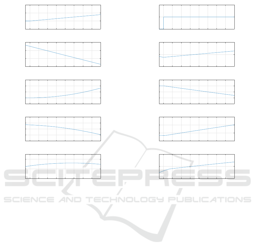
3.2.3 The System Response to Small Variations
Effect of Inlet Slurry Flow Rate Small Variation.
In order to study the response of the system to in-
puts’ small variations, the inlet slurry flow rate (F
ps1
)
is increased by 3% of the initial value (Fig. 12). By
increasing F
ps1
, the mixing tank level and the outlet
slurry flow rate increase but with a slight evolution,
SIMULTECH 2019 - 9th International Conference on Simulation and Modeling Methodologies, Technologies and Applications
32

300 400 500 600 700 800 900 1000 1100
Time (s)
0
100
200
300
Flow (m3/h)
Inlet water flow rate (Fw)
300 400 500 600 700 800 900 1000 1100
Time (s)
6
6.2
6.4
6.6
Level (m)
Mixing tank level (Lm)
300 400 500 600 700 800 900 1000 1100
Time (s)
1560
1580
1600
1620
Density (Kg/m3)
Outlet slurry density (dps2)
300 400 500 600 700 800 900 1000 1100
Time (s)
306
308
310
312
314
Flow (m3/h)
Outlet slurry flow rate (Fps2)
300 400 500 600 700 800 900 1000 1100
Time (s)
820
825
830
Speed (rpm)
Motor speed (wp)
Figure 11: The effect of water flow rate large variation.
without impacting the other outputs. However, this in-
crease of level will surely have an impact on the static
head of the system in a long-term and subsequently
an important impact on the outputs (3.2.2).
Effect of Inlet Slurry Density Small Variation.
Increasing the inlet slurry density by 3% of the initial
value, the outlet slurry density, the outlet slurry flow
rate and the mixing tank level vary slightly (Fig. 13).
However, this confirms the indirect impact of the inlet
density on the level and on the outlet slurry flow rate
even for small variations.
Effect of Inlet Water Flow Small Variation. Fig.
14 shows the effect of the inlet water flow rate small
variation on the system outputs. By adding water, the
level starts to increase, the density decreases as d
w
<
d
ps1
and the outlet slurry flow rate starts to increase
as a result of level and density changes. Thus, even a
slight variation impacts the outputs.
300 400 500 600 700 800 900 1000 1100
Time (s)
290
300
310
320
Flow (m3/h)
Inlet slurry flow rate (Fps1)
300 400 500 600 700 800 900 1000 1100
Time (s)
6.01
6.015
6.02
6.025
Level (m)
Mixing tank level (Lm)
300 400 500 600 700 800 900 1000 1100
Time (s)
1590
1600
1610
Density (Kg/m3)
Outlet slurry density (dps2)
300 400 500 600 700 800 900 1000 1100
Time (s)
306.76
306.78
306.8
Flow (m3/h)
Outlet slurry flow rate (Fps2)
300 400 500 600 700 800 900 1000 1100
Time (s)
826.35
826.4
826.45
826.5
Speed (rpm)
Motor speed (wp)
Figure 12: The effect of inlet slurry flow rate small varia-
tion.
4 CONCLUSION
The study puts forward a dynamic model and a simu-
lation for a slurry mixing and pumping process. The
dynamic model of the centrifugal pump takes into ac-
count its different parts: the hydraulic application, the
hydraulic part and the induction motor. In addition
to that, the proposed model takes the slurry density
into consideration. Therefore, the applicability of the
model is extended to other slurry types.
In order to determine the parameters of the pump
head and load torque equations, a practical method
is used based on the pump’s graphical experiments
schemes. Regarding the simulation of the process,
it is conducted using level 2 Matlab s-fucntions and
simulink environment.
According to the developed model and the simula-
tion results, it is clear that both the mixing tank level
and the slurry density impact the outlet slurry flow
rate. With regard to the slurry density effect, it di-
rectly impacts the pump torque, then the pump torque
Dynamic Modeling and Simulation of a Slurry Mixing and Pumping Process: An Industrial Case
33

300 400 500 600 700 800 900 1000 1100
Time (s)
1550
1600
1650
1700
Density (Kg/m3)
inlet slurry density (dps1)
300 400 500 600 700 800 900 1000 1100
Time (s)
6.005
6.01
6.015
6.02
Level (m)
Mixing tank level (Lm)
300 400 500 600 700 800 900 1000 1100
Time (s)
1599
1600
1601
1602
1603
Density (Kg/m3)
Outlet slurry density (dps2)
300 400 500 600 700 800 900 1000 1100
Time (s)
306.5
306.6
306.7
306.8
Flow (m3/h)
Outlet slurry flow rate (Fps2)
300 400 500 600 700 800 900 1000 1100
Time (s)
826.2
826.4
826.6
Speed (rpm)
Motor speed (wp)
Figure 13: The effect of inlet slurry density small variation.
affects the induction motor speed, then a change of the
induction motor speed changes the outlet flow rate.
That highlights the importance of these parameters in
the control strategy design.
Further research will be pursued to model the non
perfect mixture inside the mixing tank and to propose
new methods to control pumping slurry flow rate in
presence of slurry density variations.
REFERENCES
Bachus, L. and Custodio, A. (2003). Know and understand
centrifugal pumps. Elsevier.
Blevins, T. L. and Nixon, M. (2010). Control Loop Foun-
dation: Batch and Continuous Processes. ISA.
Chan, T. F. and Shi, K. (2011). Applied intelligent control
of induction motor drives. John Wiley & Sons.
Chiasson, A. D. (2016). Geothermal heat pump and heat
engine systems: Theory and practice. John Wiley &
Sons.
Deng, S. Y. (2002). Nonlinear & linear mimo control of
an industrial mixing process. Master’s thesis, McGill
University.
300 400 500 600 700 800 900 1000 1100
Time (s)
0
10
20
Flow (m3/h)
Inlet water flow rate (Fw)
300 400 500 600 700 800 900 1000 1100
Time (s)
6.01
6.02
6.03
Level (m)
Mixing tank level (Lm)
300 400 500 600 700 800 900 1000 1100
Time (s)
1597
1598
1599
1600
1601
Density (Kg/m3)
Outlet slurry density (dps2)
300 400 500 600 700 800 900 1000 1100
Time (s)
306.7
306.8
306.9
307
Flow (m3/h)
Outlet slurry flow rate (Fps2)
300 400 500 600 700 800 900 1000 1100
Time (s)
826.4
826.5
826.6
Speed (rpm)
Motor speed (wp)
Figure 14: The effect of water flow rate small variation.
El-Emam, N., Kamel, A., El-Shafei, M., and El-Batrawy, A.
(2003). New equation calculates friction factor for tur-
bulent flow on non-newtonian fluids. Oil & gas jour-
nal, 101(36):74–74.
Green, D. W. and Perry, R. H. (1997). Perry’s Chemical
Engineers’ Handbook/edici
´
on Don W. Green y Robert
H. Perry. Number C 660.28 P47 2008.
Hougen, O. A., Watson, K. M., and Ragatz, R. A. (1954).
Chemical Process Principles: Material and Energy
Balances, volume 1. John Wiley & Sons.
Isermann, R. (2007). Mechatronic systems: fundamentals.
Springer Science & Business Media.
Kallesøe, C. S., Cocquempot, V., and Izadi-Zamanabadi, R.
(2006). Model based fault detection in a centrifugal
pump application. IEEE Transactions on Control Sys-
tems Technology, 14(2):204–215.
Kallesøe, C. S., Izaili-Zamanabadi, R., Rasmussen, H., and
Cocquempot, V. (2004). Model based fault diagno-
sis in a centrifugal pump application using structural
analysis. In Proceedings of the 2004 IEEE Inter-
national Conference on Control Applications, 2004.,
volume 2, pages 1229–1235 Vol.2.
Manekar, G. and Bodkhe, S. B. (2013). Modeling Methods
of Three Phase Induction Motor. National Conference
on Innovative Paradigms in Engineering & Technol-
ogy, pages 16–20.
SIMULTECH 2019 - 9th International Conference on Simulation and Modeling Methodologies, Technologies and Applications
34

Matko, D., Geiger, G., and Werner, T. (2001). Mod-
elling of the pipeline as a lumped parameter system.
AUTOMATIKA-ZAGREB-, 42(3):177–188.
Menon, S. (2004). Piping calculations manual. McGraw
Hill Professional.
Miedema, S. (1996). Modeling and simulation of the dy-
namic behavior of a pump/pipeline system. In 17th
Annual Meeting & Technical Conference of the West-
ern Dredging Association. New Orleans.
Nienow, A. W., Edwards, M. F., and Harnby, N. (1997).
Mixing in the process industries. Butterworth-
Heinemann.
Seborg, D. E., Mellichamp, D. A., Edgar, T. F., and
Doyle III, F. J. (2010). Process dynamics and control.
John Wiley & Sons.
Skogestad, S. (2008). Chemical and Energy Process Engi-
neering. CRC Press.
Trzynadlowski, A. M. (2000). Control of induction motors.
Elsevier.
Valtr, J. (2017). Mass Flow Estimation and Control in Pump
Driven Hydronic Systems. Master’s thesis, Czech
Technical University, Czech Republic.
Wright, T. and Gerhart, P. (2009). Fluid machinery: appli-
cation, selection, and design. CRC press.
Dynamic Modeling and Simulation of a Slurry Mixing and Pumping Process: An Industrial Case
35