A Quality-based ETL Design Evaluation Framework
Zineb El Akkaoui
1
, Alejandro Vaisman
2
and Esteban Zim
´
anyi
2
1
SEEDS Team, INPT Lab, Rabat, Morocco
2
CoDE Lab, Universit
´
e Libre de Bruxelles, Brussels, Belgium
Keywords:
ETL processes, Data Integration Performance, Design Quality, Theoretical Validation, Empirical Validation.
Abstract:
The Extraction, Transformation and Loading (ETL) process is a crucial component of a data warehousing
architecture. ETL processes are usually complex and time-consuming. Particularly important (although over-
looked) in ETL development is the design phase, since it impacts on the subsequent ones, i.e., implementation
and execution. Addressing ETL quality at the design phase allows taking actions that can have a positive and
low-cost impact on process efficiency. Using the well-known Briand et al. framework (a theoretical validation
framework for system artifacts), we formally specify a set of internal metrics that we conjecture to be corre-
lated with process efficiency. We also provide empirical validation of this correlation, as well as an analysis of
the metrics that have stronger impact on efficiency. Although there exist proposals in the literature addressing
design quality in ETL, as far as we are aware of, this is the first proposal aimed at using metrics over ETL
models to predict the performance associated to these models.
1 INTRODUCTION
A data warehouse (DW) is a data repository that con-
solidates data coming from multiple and heteroge-
neous sources, in order to be exploited for decision-
making. This consolidation is performed through a
collection of processes denoted Extraction, Transfor-
mation and Loading (ETL). ETL development is usu-
ally composed of four phases, shown in Fig. 1 (Inmon,
2002). It has been widely argued that the ETL process
is complex and time-consuming, at a the point that
roughly 80% of a DW project is due to this phase (In-
mon, 2002; A. Simitsis and Sellis, ).
ETL processes are typically implemented as SQL
or Java programs orchestrated to answer organiza-
tion requirements. Thus, ETL optimization cannot
be reduced to SQL query optimization as usual in
databases: it should also take into account the process
structure. Structural optimization must manage two
main aspects: tasks combination and order. The latter
has been studied in (A. Simitsis and Sellis, 2005) as a
state space problem where, by changing the order of
the process tasks, an algorithm finds the process al-
ternative providing the best execution. However, the
combination aspect has not been covered in the lit-
erature. This factor is also relevant, since to tackle
the same integration problem, several process alter-
natives are possible, having different number of tasks
and work combinations (e.g., a process containing
few tasks, each one performing heavy work, can be
equivalent to a process that contains many less loaded
tasks). Comprehensive approaches aimed at finding
the best process structure are still lacking.
A line of research oriented towards enhancing
the ETL process proposes conceptual modeling lan-
guages to define ETL workflows (Z. El Akkaoui
and Zim
´
anyi, 2012; Trujillo and Luj
´
an-Mora, 2003;
P. Vassiliadis and Skiadopoulos, ), sometimes pre-
sented together with ETL design guidelines (U. Dayal
and Wilkinson, 2009). We comment on these propos-
als in Section 2. Most of them propose metrics that
can lead to improve characteristics like usability and
maintenance. However, to the best of our knowledge,
no work has studied and validated ETL model design
criteria with respect to the crucial issue of ETL pro-
cess efficiency.
To provide a solution to this problem, in this pa-
per we present tools that, based on the ETL design
characteristics, can help to predict the efficiency of
the process. We do this by means of a set of structural
(also denoted internal) metrics, defined based on the
Briand et al. (L. Briand and Basili, 1996) theoretical
framework in order to guarantee the mathematical va-
lidity of the approach. The nice property of these met-
rics is that they can be computed at design time, and
that, as we will show, they are correlated with ETL ef-
El Akkaoui, Z., Vaisman, A. and Zimányi, E.
A Quality-based ETL Design Evaluation Framework.
DOI: 10.5220/0007786502490257
In Proceedings of the 21st International Conference on Enterprise Information Systems (ICEIS 2019), pages 249-257
ISBN: 978-989-758-372-8
Copyright
c
 2019 by SCITEPRESS – Science and Technology Publications, Lda. All rights reserved
249

Figure 1: Development steps & improvement criteria.
ficiency, specifically with the process throughput (an
external metric). Therefore, proving the correlation
stated above is an important achievement in ETL de-
sign, since, given a collection of alternative ETL mod-
els, it would allow predicting the one that is likely to
deliver the best performance without actually needing
to code a single line, dramatically dropping the costs
of the DW project.
The paper is organized as follows. Section 2 dis-
cusses related work. Section 3 presents our running
example, while in Section 4 we introduce the formal
data model for the ETL process graph. Section 5 stud-
ied the internal and external measures used to evaluate
the design quality of the ETL model. Section 6 reports
the experimental validation and its results, concluding
in Section 7.
2 RELATED WORK
A quality model (e.g., (B. Boehm and Merritt, 1978))
defines a set of quality goals together with a set of
practices for achieving and evaluating them. The
ISO/IEC 9126 standard
1
provides a standard qual-
ity model for software products. Built on soft-
ware quality approaches, ETL process quality eval-
uation methods have been proposed. These proposals
mainly address ETL usability or maintainability eval-
uations. Quality evaluations for ETL design proposed
in (L. Mu
˜
noz and Trujillo, 2010; P. Vassiliadis and
Skiadopoulos, ) derive measures based on the Briand
et al. (L. Briand and Basili, 1996) evaluation frame-
work. While Vassiliadis et al. (P. Vassiliadis and Ski-
adopoulos, ) limit to propose supposedly useful mea-
sures for ETL models, Mu
˜
noz et al. (L. Mu
˜
noz and
Trujillo, 2010) validate the measures empirically by
studying their effect over two ISO quality dimensions,
namely usability and maintenance. Further (Z. El
Akkaoui and Trujillo, 2013; G. Papastefanatos and
Vassiliou, 2009) cover maintainability and support
data source evolution.
Enhancing ETL efficiency at the implementation
step has been studied in some few works. Simitsis et
al. (A. Simitsis and Dayal, 2013) proposes an opti-
1
http://www.iso.org/iso/iso catalogue/catalogue tc/
catalogue detail.htm?csnumber=22749
(a)
(b)
Figure 2: (a) Tables from source database; (b) Location hi-
erarchy.
mizer that converts the logical flow to an executable
form that is optimized for the underlying infrastruc-
ture according to user-specified objectives. Another
optimization approach (A. Simitsis and Dayal, 2012)
intends to avoid bad execution plans by partitioning
the original data model into submodels that we run
on each engine. Another contribution (T. Majchrzak
and Kuchen, 2011), by defining a set of performance
measures, a comparison is made between Talend (a
code generation-based tool) and Pentaho (an engine-
based tool). Results showed that Talend is more effi-
cient in terms of execution time and CPU usage, while
Pentaho is less memory-consuming. Further, (Ali
and Wrembel, 2017; G. Kougka and Simitsis, 2018)
survey almost aforementioned data flow optimization
techniques. But (G. Kougka and Simitsis, 2018)
expands the study to various other data-centric flow
topics besides ETL processes, including database en-
gines, MapReduce systems, and business processes.
In the present work we go further than existing pro-
posals, quantitatively assessing the relationship be-
tween a set of design quality metrics evaluated over
the structure of the ETL process model, and external
metrics obtained at execution time.
3 RUNNING EXAMPLE
To model a DW we use the well-known star-
schema (Kimball and Ross, 2002), where DW tables
are of two kinds: dimension and fact tables. Dimen-
sions actually represent aggregation hierarchies along
which fact data are summarized. ETL processes take
data from the sources into the star-schema tables. To
illustrate our evaluation framework, we use a portion
ICEIS 2019 - 21st International Conference on Enterprise Information Systems
250

of an ETL process that loads a collection of dimension
tables containing customer and location data. Fig. 2b
shows dimension tables DimArea, DimCountry, Dim-
State, and DimGeography. The first three ones are
populated using an XML file denoted Territories.xml.
DimGeography is populated using geographical data
with attributes City, State, ZipCode, and Country,
present in the Customer and Supplier tables of the
Northwind database
2
(Fig. 2a). Before populating the
Location hierarchy, the geography data needs some
cleansing and transformation operations to fit the data
warehouse requirements, namely: (a) Data comple-
tion, which requires dealing with null values. For
example, the attribute State may be null in the Cus-
tomer and Supplier source tables. The ETL process
fixes this by using an external source file Cities.txt,
which contains three fields: city, state, and country.
(b) Data consolidation. For example, in the source
databases, attribute State contains either a state name
(e.g., California) or a state code (e.g., CA). In the lat-
ter case, the state code is either left empty or con-
verted into the state name using the State table with at-
tributes StateId, StateName, and Code (the ISO stan-
dard code), which contains the link between the state
name and its code. (c) Consistency, in particular with
respect to referential integrity constraints. During the
loading of the data into the data warehouse, referen-
tial integrity between all the hierarchy tables must be
ensured.
To model complex processes, several concep-
tual modeling tools (mentioned in Sections 1 and 2)
have been proposed in the literature. In this paper
we use an ETL model based on BPMN4ETL (El
Akkaoui and Zim
´
anyi, 2012), which models ETL pro-
cesses as workflows, extending the BPMN notation.
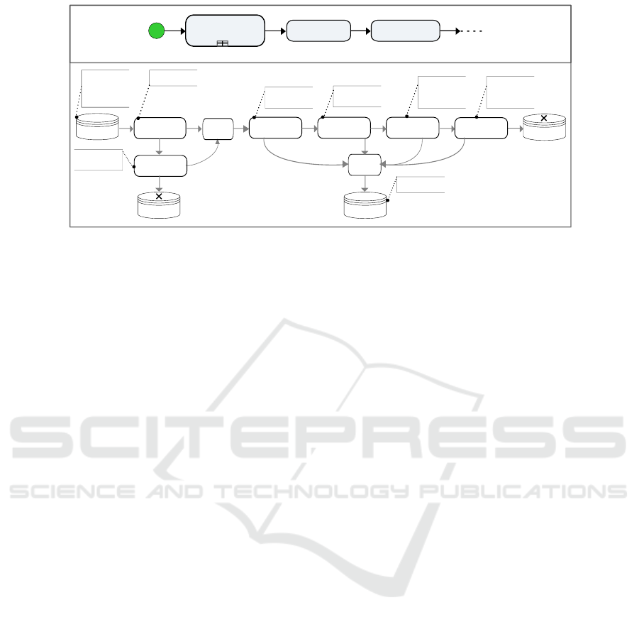
Fig. 3 shows the loading process for the DimGeog-
raphy dimension of our running example, modeled
in BPMN4ETL. More in detail, an ETL model in
BPMN4ETL is perceived as composed of a control
process containing several data processes. A control
process (top process of Fig. 3) manages the coarse-
grained groups of tasks and/or sub-processes, while a
data process (bottom processes of Fig. 3) operates at
finer granularity, detailing how input data are trans-
formed and output data are produced. For exam-
ple, populating each fact (dimension, view, tempo-
rary, etc.) table in the data warehouse constitutes a
data process, whereas sequencing the load of differ-
ent dimension levels constitutes a control process.
2
http://www.microsoft.com/en-us/download/details.
aspx?id=23654
4 DATA AND QUALIY MODELS
4.1 ETL Data Process Graph
We now present the ETL model we use in this pa-
per. Due to space limitations we restrict ourselves to
study the data process perspective, which constitutes
the portion of the ETL process where transformations
occur, and we do not deal with the control process.
There is T, a set of node types. T = {“data input”,
“data output”, “filter”, “field lookup”, “field deriva-
tion”, “field generation”, “join”, “union”, “aggrega-
tion”, “sort”, “pivot”, “script”}. There is also a set A
containing a list of possible actions performed by a
node. A = {“field manipulation”, “field generation”,
“join”, “lookup”, “branching”, “extraction”, “load”},
where “field manipulation” action covers field com-
putation, deletion, addition, sorting, pivoting, and
splitting. In addition, a node has a traversing stream.
The input stream of a node has schema:
(( f ield
1
, f ield
1
.datatype), ..., ( f ield
i
, f ield
i
.
datatype))
Definition 1 (Data Process Graph (DPG)). A data
process graph is a directed graph G(N,E) where N =
n
1
, n
2
, ..., n
p
is the set of nodes representing the data
tasks, and E = e
1
, e
2
, ..., e
q
is the set of edges between
nodes. An edge e = (a, b) ∈ E means that b receives
data from node a for further processing. In addition,
the following holds:
• There is a function with signature N 7→ T, that
maps a node n to its type.
• Each node has an associated set of actions, which
is a subset of A. There is a relation actions ∈ N ×
A, reflecting this association.
• A relation schema ∈ N × S defines the input fields
of a node.
• A node belongs to a flow category. It is either a
branching node: “filter”, a join node: “join”, a
union node, a lookup node: “fieldlookup” or a
unitary node, for the other nodes.
• A node belongs to a script category. It is either a
script node “script”, or a non-script node. In ad-
dition, “datainput” and “fieldlookup” nodes can
also be considered script nodes when they include
a data extraction script. Otherwise, they are con-
sidered non-script nodes.
• A node belongs to a stream category accord-
ing to the applied treatment on its traversing
data. It is either a row-by-row node (“field
derivation”, “field generation”), a row-set node
(“sort”, “pivot”, “aggregation”), or an input-
output node (“data input”, “data output”). Row-
by-row nodes are asynchronous (each row is pro-
A Quality-based ETL Design Evaluation Framework
251

Filter
FieldLookup
DataInput
SelectQuery
Supplier
Customer
State = Null
Union
DataOutput
DimGeography
FieldLookup FieldLookup FieldLookup FieldLookup
Union
DataOutput
Found
Not
Found
Not
Found
Not
Found
Not
Found
Cities.txt
State
Not null
Null
DataOutput
Not
Found
Found
Found
DimState.
StateName
DimState.
StateEnglishName
DimCountry.
StateCode
CountryName
DimCountry.
StateCode
CountryCode
n
1
n
2
n
3
n
4
n
5
n
6
n
7
n
8
n
9
n
10
n
11
n
12
DimArea Dim State
DimCountry Load
Start
Event
DimCustomerDimGeography
Control Process
Data Process
Figure 3: DimGeography load data processes.
cessed when it arrives), while row-set nodes are
synchronous (processing starts only when the
whole row-set arrives).
• Data annotations can be associated to nodes and
edges as free text.
Definition 2 (Valid Data Process Graph). A Data Pro-
cess graph G is valid if the following constraints hold:
• G has at least two nodes: a “data input” node
and a“data output” node.
• Each node in G respects the allowed in- and out-
degrees, predefined according to its type.
• Each node in G has at least one predecessor ex-
cept for the “data input” nodes.
• Each node performs a number of actions. Script
nodes have no predefined number of actions,
while non-script nodes have one action.
The ETL process in Fig. 3 depicts a graph with
12 nodes. According to the definitions below, the
node n
1
= DataInput, is a unitary, non-script, and row-
by-row node, such that type(n
1
) = “data input”, and
actions(n
1
) =“extraction”.
4.2 Measure Families
Quality concepts like complexity, coupling, cohesion
or size are very often subject to interpretation. Thus,
Briand et al. (L. Briand and Basili, 1996) pro-
posed a framework facilitating the definition of qual-
ity measures based on mathematical properties. This
guides the designer in creating mutli-aspect and non-
redundant measures. The authors proposed a set of
mathematical properties general enough to be appli-
cable to a wide set of artifacts, not only programming
code. We next show how the proposal can be applied
to the ETL process context.
The framework defined by Briand et al. identi-
fies the following families of measures, which also
can be called quality dimensions (each family allows
creating a collection of associated measures that ‘op-
erationalize’ the concept): (a) Size: reflects the num-
ber of elements in a system; (b) Coupling: measures
the strength of the connections between system el-
ements; (c) Cohesion: characterizes the interaction
between elements in sub-systems or modules. It as-
sesses the tightness with which related program fea-
tures are grouped together in sub-systems or mod-
ules. A highly cohesive system has few interactions
between its elements; (d) Complexity: in general it
is used for assessing complex system behavior. It in-
forms about the effort needed to maintain, change and
understand a system. Complexity is a system property
that depends on the relationships between elements,
rather than a property of an isolated element.
Fig. 4a depicts the modular system decomposition
borrowed from (L. Briand and Basili, 1996), and its
correspondence with the DPG of Definition 1. The
modular system includes modules that contain ele-
ments. A system is a tuple < N, E > where N is the
set of elements of the system, and E is the set of edges
between the elements. A module m is a subset of the
elements of the system. In general, modules can over-
lap. When the modules partition the nodes in a sys-
tem, then this system is called modular. The DPG
corresponds to a modular system where nodes corre-
spond to modules and actions to elements.
By definition, size and complexity measures are
computed over the whole modular system, while the
other measures are computed over modules compos-
ing this modular system. Following (L. Briand and
Basili, 1996), the measures belonging to a family
must verify a set of properties, e.g.:
• Non-negativity: the measure must not be in-
versely related to the studied aspect. (Applies to
ICEIS 2019 - 21st International Conference on Enterprise Information Systems
252

(a) (b)
Figure 4: (a) The structure of a system in (L. Briand and Basili, 1996); (b) Its mapping to the DPG.
Size, Coupling and Complexity).
• Null value: the measure must be null when a sys-
tem does not contain any element. (Applies to the
measures in the four families).
• Additivity: when several modules do not have el-
ements in common, the size of the system is the
size of its modules. (Applies to Size).
• Non-negativity and normalization: the measure is
independent of the size of the system or module,
and belongs to a certain interval. (Applies to Co-
hesion).
• Monotonicity: states that adding internal relation-
ships in modules does not decrease a measure’s
value (however, adding an edge between modules
decreases the measure). (Applies to Coupling and
Cohesion).
From Definition 1 we can devise the node clas-
sification hierarchy of Fig. 4b. At the bottom of
this classification, we identify seven node categories.
Actually, the rationale behind these seven size mea-
sure categories is that we conjecture that these cate-
gories impact on efficiency (we validate this in Sec-
tion 6). Moreover, Fig. 4b shows the relationship be-
tween the graph definition and the measure families
in (L. Briand and Basili, 1996). For example, the Ac-
tion category is related to the Cohesion family. The
other node categories are linked to the Size family.
In our approach, we consider a DPG as a modu-
lar system, where a node is a module, an edge is the
inter-module relationship, and actions are the module
elements. Hence, size measures are defined over the
whole graph, and cohesion measures are defined over
its modules. The cohesion measure is aimed at reflect-
ing the intra-module interactions between elements
within modules (actions). No coupling and complex-
ity measures are defined because coupling is an inter-
module relationship, and there is no inter-module in-
teraction among their elements (actions). Complex-
ity is linked to the inter-module relationships, and be-
cause of the DPG structure, the size measures also
inform about the complexity.
5 ETL DESIGN QUALITY
MEASURES
Efficiency is an ISO 9126 quality dimension that eval-
uates the capability of a model to provide appropri-
ate performance relative to the amount of resources
used, under stated conditions. In this section we first
present efficiency (external) measures from the ISO
9126 (Becker, 2008), typically used to compute the
ETL process performance. Then, based on the mea-
sure families studied in Section 4, we propose a set of
structural (internal) measures, particularly describing
the graph node combination, to be applied at the de-
sign level. These internal measures are likely to im-
pact the ETL process efficiency.
5.1 External Measures
The ISO 9126 quality dimensions include function-
ality, reliability usability, efficiency, maintainability,
and portability. The set of measures proposed by the
ISO standard to evaluate ETL execution efficiency are
depicted in Table 1. For example, Execution Time
(ET) is the server time required to complete the exe-
cution of an ETL process. A more significant measure
to evaluate ETL efficiency is Throughput (Th), which
takes into account the size of the data processed by the
ETL system. The throughput is computed as the num-
ber of rows per unit of time processed. Additional
performance measures address resource usage. For
example, the Disk I/O computes the number of disk
readwrite actions performed during the ETL execu-
tion. Note that the evaluation of the external measures
require a complete implementation and execution of
the ETL process.
A Quality-based ETL Design Evaluation Framework
253

Table 1: External measures.
Measure Name Description
ET Execution
Time
Time the server takes to complete the
execution
NL Network
Latency
Time the network takes to transfer data
from data sourcetarget to the data stag-
ing
Th Throughput Size of data served by the ETL model
per unit of time
DIO Disk IO Number of disk readwrite
Me Memory Memory amount usage
5.2 Internal Measures
We next propose a collection of internal measures,
formalize them, and show that they satisfy the proper-
ties defined in (L. Briand and Basili, 1996). We base
the definition of the internal measures in the formal
definition of a DPG (Definition 1). To represent the
framework in (L. Briand and Basili, 1996), we call G
= (N, E) a graph, and m = (N
1
, E
1
) a module in G,
such that a set of nodes N
1
is linked with edges E
1
such that N
1
⊆ N, and E
1
⊆ E. A module can include
only one node.
Size Family. It appears straightforward to assume
that the larger the graph size, the lesser the efficiency
we can expect from an ETL process, and that each ad-
ditional node will increase the execution time and/or
resource usage. Importantly, the data processing of a
decomposed ETL graph are delayed by the data trans-
fer time between nodes. In addition, a decomposed
graph has a latency time due to different transforma-
tions (instead of a single combined transformation)
applied over each row. As mentioned in Definition
1, a node belongs to a stream category according to
the way it is processed (row-by-row, row-set or input-
output). A higher latency is hence expected for de-
composed row-set nodes. For this reason, we define a
size measure for each node category since we expect
that each has a specific influence on the efficiency. We
next define the measures in the Size family.
Definition 3 (Branching Nodes). Given a graph G.
The Branching Nodes measure of G, BN(G), is the
number of branching nodes in G. It is computed as
the cardinality of the nodes in the “branching” cate-
gory:
BN(G) = card({n ∈ N | type(m) ∈
“ f ilter”}})
Definition 4 (Joining Nodes). Given a graph G, the
Joining Node measure of G, JN(G), is the number of
node in the “joining” category:
JN = card({n ∈ N | type(m) ∈
{“ join”, “union”}})
Definition 5 (Lookup Nodes). Given a graph G, the
Lookup Nodes measure of G, LN(G), is the number of
nodes in G belonging to the “lookup” category and
which perform only one action (it does not include
scripts).
LN(G) = card({n ∈ N | type(m) ∈
{“ f ieldlookup”} ∧ card(actions(n)) = 1})
Definition 6 (Script Nodes). Given a graph G, the
Script Nodes measure of G, SN(G), is the number of
script nodes in the module m, and it is computed as
the cardinality of the nodes having a number of ac-
tions greater than 2.
SN(G) = card({n ∈ N | card(actions(n))
≥ 2})
Example 1. For G= DimGeography in Fig. 3, we
have:
BN(G) = card({n
2
}) = 1.
JN(G) = card({n
3
, n
11
}) = 2.
LN(G) = card({n
4
, n
5
, n
6
, n
7
, n
9
}) = 5.
SN(G) = card({n
1
, n
6
, n
7
}) = 3.
Finally, we define three measures on the stream
category. The more resource-consuming stream type
is the row-set type because it implies a blocking strat-
egy that delays the execution, in particular when deal-
ing with large data volumes. The row-by-row type
is less time-consuming. The input-output type is in
charge of importing and exporting data from and to
databases.
Definition 7 (RS, RbR, and IO Nodes). Given a
graph G, the Row-Set (RS) Nodes measure
RSN(G) = card({n ∈ N | type(n) ∈
{“sort”, “pivot”, “aggregation”}})
The Row-by-Row (RbR) Nodes measure of G,
RbRN(G), is the number of row-by-row nodes in G.
RbRN(G) = card({n ∈ N | type(n) ∈ {
“ f ieldderivation”, “ f ieldgeneration”}})
The Input-Output (IO) Nodes measure of G,
ION(G), is the number of data input and data output
nodes in G.
ION(G) = card({n ∈ N | type(n) ∈
{“datainput”, “dataout put”}
and card(actions(n)) = 1})
Example 2. For G = DimGeography graph of Fig. 3,
we have: RSN(G) = 0 (G does not contain any row-set
node), RbRN(G) = 0 (G does not contain any row-by-
row node), and ION(G) =
card({n
1
, n
8
, n
10
, n
12
}) = 4.
ICEIS 2019 - 21st International Conference on Enterprise Information Systems
254

The mathematical properties that must character-
ize any size measure are verified by the proposed ones
as shown next (proofs omitted).
1. Non-negativity. Meaning that for any graph G,
BN(G) ≥ 0, JN(G) ≥ 0, LN(G) ≥ 0, SN(G) ≥
0, RSN(G) ≥ 0 RbRN(G) ≥ 0, and ION(G) ≥ 0;
2. Null value, implying that if G = ∅ =⇒ BN(G) =
0, JN(G) =0, LN(G) = 0, SN(G) = 0, RSN(G) = 0
RbRN(G) = 0, and ION(G) = 0;
3. Module additivity, having m
1
=< N
m1
, E
m1
> and
m
2
=< N
m2
, E
m2
> it holds that (m
1
⊆ G and m
2
⊆
G and N = N
m1
∪ N
m2
and N
m1
∩ N
m2
= ∅) =⇒
BN(G) = BN(m
1
)+BN(m
2
), JN(G) = JN(m
1
)+
JN(m
2
), ...
It is worth mentioning that in our graph system,
a module is a unitary node sub-system, therefore
N
m1
contains only one node.
Size measures inform about the high-level orga-
nization of the work in the graph. We need a com-
plementary characteristic in order to quantify the dis-
tribution of the work through the graph nodes. We
define it next.
Cohesion Family. Cohesion is related to the amount
of work processed by the graph nodes. Depending
on the scripting category, some nodes may perform
more actions than other ones. In particular, script,
field lookup, and data input nodes can perform a large,
unpredictable, amount of actions. The Cohesion Ac-
tion measure, defined next, is aimed at reflecting the
amount of work carried out by such nodes. We ex-
pected that nodes with a low cohesion (i.e., perform-
ing more actions) consume more time and resources
than nodes with a high cohesion. Note that this mea-
sure is defined for each system module or node.
Definition 8 (Cohesion Action). Given a module m =
< N, E > from a graph G, the Cohesion Action mea-
sure of m, CA(m), is defined as:
CA(m) =
LCAN(m)
CAC(G)
where CAC =
∑
n∈N
card(actions(n)) and
LCAN =
∑
n∈N
card(actions(n)) s.t. actions(n) ≥ 2
CA(m) is the proportion of low cohesion nodes in the
graph G. It determines the participation of each node
in performing the work. CAC(m) is the number of all
actions performed by the nodes in G. It estimates the
work produced by the whole graph. LCAN(m) is the
cardinality of the actions of low cohesion nodes.
Example 3 (Cohesion Action). For our example
graph, n
1
, n
6
, n
7
are low cohesion nodes. Node n
1
is a “data input” node using a script which applies
both, extraction and join actions (annotated e, j as
specified by the set of actions A in Definition 1). Also,
n
6
and n
7
are “field lookup” nodes containing a join
script in their lookup condition (annotated lk, j).
CAC(G) = card({e, j}) + 4 × card({lk}) +
2 × card({lk, j}) + 3 × card({l}) + 2 × card({ j})=
15;
LCAN({n
1
}) = card({ j, e}) = 2; LCAN({n
6
}) =
card({b, j}) = 2;
LCAN({n
7
}) = card({c, j}) = 2;
CA({n
1
}) = CA({n
6
}) = CA({n
7
}) = 2/15 =0.13.
The mathematical properties that must be accom-
plished by any cohesion measure are verified by CA,
that are not been demonstrated due to space limita-
tion.
6 EXPERIMENTAL VALIDATION
In this section, we describe a set of experiments aimed
at providing a preliminary empirical validation of the
relationship between the proposed internal measures,
and the external measure Throughput (Th). We chose
Th as the external measure since it can be computed
using the execution elapsed time extracted from the
system’s log file, allowing obtaining meaningful re-
sults. Our hypotheses are:
• H1: The number of join, lookup, script, row-set,
and input-output nodes are correlated with Th;
• H2: The number of row-by-row nodes has low im-
pact on the Th;
• H3: Adding branching nodes does not decrease
Th;
• H4: The best script node form is the data input
node using a script. This is better than using a
specific script node.
• H5: For optimization purposes, replacing join
nodes with a data input script node increases Th.
On the contrary, replacing lookup nodes with data
input script nodes is not beneficial for throughput.
The validation of these hypothesis will guide the
ETL designer in answering fundamental questions
such as: which construct should I use to optimally add
a specific ETL transformation? What are the design
criteria that are increasing or decreasing the through-
put? Given two graphs, can we anticipate on which
one will have the best throughput?
A Quality-based ETL Design Evaluation Framework
255

6.1 Experimental Setting
We ran our experiments using Microsoft’s SQL
Server Integration Services (SSIS)
3
, over a com-
puter equipped with an Intel Dual-Core processor at
2.10GHz and 4 Gigabytes of RAM running Windows
7 OS.
The internal measures to be evaluated may influ-
ence on each other. At this point we are interested
in finding out the relation between a single variable
(measure) and Th. Thus, we performed a set of con-
trolled experiments, in order to detect the individual
impact over Th of each internal design factor. We cre-
ated 54 graphs in the following way: we defined an
initial ETL model using BPMN4ETL, and translated
the graph to a data flow SSIS component. To analyze
each measure we modified the initial graph by modi-
fying the combination of nodes (ETL tasks). For ex-
ample, to study the influence of the number of branch-
ing nodes (measure BN), we started with a combina-
tion of the graph having BN = 1, and then we increase
BN by adding neutral branching nodes to obtain seven
graphs with BN = 1, 3, 5, 8, 10, 15, and 20. We
performed the same with join nodes, lookup nodes,
script nodes, row-by-row nodes, row-set nodes, input-
ouput nodes. To assess cohesion action we created 7
graphs with different number of actions in data input
and script nodes. All these yielded 54 graphs to per-
form, basically, the same job. We measured Th for
each graph execution. In addition, and to take into
account the data size, we ran each graph for differ-
ent data sizes: the initial data source size is 56Kb,
including 290 rows. We multiplied it by 100, 500,
and 1000, producing, respectively, a data input vary-
ing from 65Kb to 65Mb. In the figures of this section,
Th is expressed in KBytes by millisecond (Kb/ms).
6.2 Discussion of Results
We now analyze the results from our experiments with
respect to the hypotheses H1 through H5. First, we
studied the correlation between each measure and Th,
for different data source sizes (1x, 100x,..). The re-
sults are depicted in Table 2, where measures are in-
dicated as BN, JN, etc. Table 2 shows that all the mea-
sures are strongly correlated to the throughput, except
for BN, JN and CA-S. For BN, this implies that an
additional branching node has a low impact on the
throughput. For the JN and CA-S measures, the very
weak throughput results reflect the low performance
of join nodes in the SSIS tool. Thus, further exper-
iments are required over different tools. All other
3
http://msdn.microsoft.com/en-us/library/ms141026.
aspx/
measures are negatively correlated to the throughput,
confirming that adding nodes decreases Th. There-
fore, as a first result, these strong correlations vali-
date our measures and confirm their influence over
the efficiency goal represented in this study by the
throughput external measure. For the CA measure we
performed two kinds of experiments: (a) adding node
actions to the data input (DI) script, yielding the CA
measure (denoted CA-DI) computed on a DI script
node; (b) adding the specific script (S) node action,
yielding the CA measure (denoted CA-S) computed
on an specific script node. The correlations for the
(CA-DI) measure were good, although no correlations
could be computed for (CA-S) because of the very
low throughput.
The second analysis, shown in Fig. 5a captures
(for the largest dataset) the throughput variation for
each measure. In the X axis we represent the number
of nodes of each type, and on the Y axis, the through-
put. Fig. 5a shows that adding all kinds of nodes
(except from branching nodes) strongly decreases Th.
Adding branching nodes does not reduce throughput,
confirming results shown in Table 2. However, adding
BNs could be beneficial for other external measures
(e.g., related with parallel execution). These results
were the same for all dataset sizes. Thus, the results
above confirm hypotheses H1 through H3.
We now analyze hypotheses H4 and H5. Fig. 5b
shows (also for the largest dataset) that script nodes
(CA-DI) can be used (whenever possible) instead of
join ones since the latter deliver worse throughput.
Analogously, we can join several input nodes in a sin-
gle script node to increase Th. Fig. 5b also shows
that lookup nodes are better than script ones. This can
be explained by the optimization capabilities provided
by the ETL server in managing such type of nodes. In
summary, our results suggest that ETL thoughput can
be enhanced if at the design stage we choose more
efficient kinds of nodes. Note, however, that this is
not always possible (e.g., it is not reasonable to group
several row-set nodes in the same script). Again, re-
sults were the same for all dataset sizes. Therefore,
hypotheses H4 and H5 are confirmed by our experi-
ments.
7 CONCLUSION
We have formally presented, and empirically vali-
dated, a collection of measures that, computed over
alternative ETL process graphs (i.e., representing dif-
ferent combinations of tasks), allow predicting how
they will perform with respect to each other before
writing even a single line of programming code. As
ICEIS 2019 - 21st International Conference on Enterprise Information Systems
256

Table 2: Correlations.
Size BN JN LI SN RSN RbRN ION CA - DI CA-S
65Kb -0.82 - -0.90 -0.93 -0.81 -0.94 -0.88 -0.97 -
6.5Mb -0.69 - -0.88 -0.74 -0.72 -0.93 -0.81 -0.97 -
32.5Mb 0.13 - -0.82 -0.62 -0.81 -0.97 -0.93 -0.96 -
65Mb 0.64 -0.51 -0.80 -0.69 -0.78 -0.99 -0.93 -1.00 -
(a) (b)
Figure 5: (a) Throughput vs. # of nodes; (b) Lookup nodes vs. join nodes vs. script nodes.
a consequence, our results allow us to draw a set of
guidelines to design efficient ETL workflows. As fu-
ture work, we will work in the assessment of the com-
plete impact over performance of the measures pro-
posed in this paper, since at this stage we focused
on the individual (partial) impact of each one of such
measures.
REFERENCES
A. Simitsis, K. W. and Dayal, U. (2013). Hybrid analytic
flows - the case for optimization. Fundamenta Infor-
maticae, pages 303–335.
A. Simitsis, K. Wilkinson, M. C. and Dayal, U. (2012). Op-
timizing analytic data flows for multiple execution en-
gines. In SIGMOD’12, 12th International Conference
on Management of Data. ACM Press.
A. Simitsis, P. V. and Sellis, T. State-space optimization
of ETL workflows. IEEE Trans. Knowl. Data Eng.,
17(10).
A. Simitsis, P. V. and Sellis, T. (2005). Optimizing ETL pro-
cesses in data warehouse environments. In ICDE’21,
21st International Conference on Data Engineering.
IEEE Computer Society Press.
Ali, S. and Wrembel, R. (2017). From conceptual design
to performance optimization of etl workflows: current
state of research and open problems. The VLDB Jour-
nal, 26(6):777–801.
B. Boehm, J. Brown, H. K. M. L. G. M. and Merritt, M.
(1978). Characteristics of Software Quality (TRW se-
ries of software technology). Elsevier.
Becker, S. (2008). Performance-related metrics in the ISO
9126 standard. In I. In Eusgeld, F. F. and Reussner,
R., editors, Dependability Metrics, pages 204–206.
Springer, Berlin, Heidelberg.
El Akkaoui, Z. and Zim
´
anyi, E. (2012). Defining ETL
worfklows using BPMN and BPEL. In DOLAP’09,
9th International Workshop on Data Warehousing and
OLAP. ACM Press.
G. Kougka, A. G. and Simitsis, A. (2018). The many faces
of data-centric workflow optimization: a survey. In-
ternational Journal of Data Science and Analytics,
6(2):81–107.
G. Papastefanatos, P. Vassiliadis, A. S. and Vassiliou, Y.
(2009). Policy-regulated management of ETL evolu-
tion. Journal Data Semantics, 5530:146–176.
Inmon, W. (2002). Building the Data Warehouse. Wiley.
Kimball, R. and Ross, M. (2002). The Data Warehouse
Toolkit, 2nd. Ed. Wiley.
L. Briand, S. M. and Basili, V. (1996). Property-based soft-
ware engineering measurement. IEEE Transactions
on Software Engineering, 22(2):68–86.
L. Mu
˜
noz, J. M. and Trujillo, J. (2010). A family of exper-
iments to validate measures for UML activity. Infor-
mation and Software Technology, 52(11):1188–1203.
P. Vassiliadis, A. Simitsis, P. G. M. T. and Skiadopoulos, S.
A generic and customizable framework for the design
of ETL scenarios. Information Systems, 30(7).
T. Majchrzak, T. J. and Kuchen, H. (2011). Efficiency eval-
uation of open source ETL tools. In SAC’11, 11th
Proceedings of the ACM Symposium on Applied Com-
puting. ACM Press.
Trujillo, J. and Luj
´
an-Mora, S. (2003). A UML-based
approach for modeling ETL processes in data ware-
houses. In ER’22, 22nd International Conference on
Conceptual Modeling. Springer.
U. Dayal, M. Castellanos, A. S. and Wilkinson, K. (2009).
Data integration flows for business intelligence. In
EDBT’09, 9th International Conference on Extending
Database Technology. ACM Press.
Z. El Akkaoui, J. Maz
´
on, A. V. and Zim
´
anyi, E. (2012).
BPMN-based conceptual modeling of ETL processes.
In DAWAK’12, 12th International Conference on Data
Warehousing and Knowledge Discovery. Springer.
Z. El Akkaoui, E. Zim
´
anyi, J. M. A. V. and Trujillo, J.
(2013). A bpmn-based design and maintenance frame-
work for ETL processes. International Journal of
Data Warehousing and Mining IJDWM, 9(3):46–72.
A Quality-based ETL Design Evaluation Framework
257