Development and Validation of Active Roll Control based on

Actor-critic Neural Network Reinforcement Learning

Matthias Bahr, Sebastian Reicherts, Philipp Maximilian Sieberg, Luca Morss and Dieter Schramm

Chair of Mechatronics, University of Duisburg-Essen, Lotharstraße 1, 47057 Duisburg, Germany

Keywords: Artificial Neural Network, Active Roll Control, Neural Controller, Reinforcement Learning, Actor-critic,

Driving Maneuvers, Vehicle Dynamics, Machine Learning.

Abstract: This paper deals with the application of machine learning for active roll control of motor vehicles. For this

purpose, a special learning method based on reinforcement learning with an actor-critic model is used. It

discusses and elaborates the basic design of the neural controller and its optimization for a fast and stable

training. The methods mentioned are then validated. Both the training and the validation data are simulatively

generated with the software environments MATLAB / Simulink and IPG CarMaker, while the architecture

and training of the artificial neural network used is realized with the framework TensorFlow.

1 INTRODUCTION

Investigations in the field of vehicle dynamics and the

development of driver assistance systems have the

goal of increasing vehicle safety and ride comfort.

Active roll stabilization is an assistance system that

enhances both vehicle safety and driving comfort. By

means of actuators, components of the chassis can be

arbitrarily influenced within their physical limits.

These actuators are variably controlled via a control

unit. The development and optimization of such

regulations is one of the main tasks in the design of

driver assistance systems. In addition to conventional

PID controlling, other control algorithms such as a

fuzzy control are possible (Sieberg et al., 2018).

Due to the relevance of machine learning in

neuroinformatic, artificial neural networks are

increasingly being used in control engineering as

well. These can either completely replace the

conventional controllers or specify setpoint values for

the regulation, which are forecasted from the process

flow of the system to be controlled. This applicability

to active roll stabilization is presented in this article.

In comparison to supervised and unsupervised

learning the application of reinforcement learning to

control tasks of vehicle dynamics is rarely researched.

Also, the presented specific method of the actor-critic

is infrequently used for control tasks. Specially, the

transfer to the application of vehicle dynamics is a

comparative unexplored science. So, the developed

model and method has a highly scientific relevance.

The focus of this paper is not on the development

of an optimized controller for perfect stabilization,

but much more on the documentation that the

developed model proves useful for controlling the roll

angle of a motor vehicle and thus for other driving

dynamics. In this case, the roll angle is to be reduced

in comparison to a passive stabilization with common

spring and damper elements. This work is aimed to

investigate the utility of the actor-critic method for

control tasks and particularly controlling vehicle

dynamics. Nevertheless, the method can be applied to

a broad spectrum of control tasks.

This article will present the approach to develop a

controller based on the actor-critic Reinforcement

Learning method. The training and validation are

accomplished within a simulation environment

including MATLAB/Simulink, IPG CarMaker and

TensorFlow. The results are validated in comparison

to a passive roll stabilization.

2 RELEVANT RESEARCH

Boada et al., (2009) have made an approach on the

active control of roll-stabilizers based on machine

learning methods. Here, a simple ANN is trained on

the simulation of a single unit heavy vehicle model

with five degrees of freedom, using RL methods. The

ANN-architecture consists of a dynamic input layer

and an output layer. The few degrees of freedom of

the model used and the very ideal training and testing

Bahr, M., Reicherts, S., Sieberg, P., Morss, L. and Schramm, D.

Development and Validation of Active Roll Control based on Actor-critic Neural Network Reinforcement Learning.

DOI: 10.5220/0007787400360046

In Proceedings of the 9th International Conference on Simulation and Modeling Methodologies, Technologies and Applications (SIMULTECH 2019), pages 36-46

ISBN: 978-989-758-381-0

conditions leave room for the development of

machine learning control for more realistic scenarios.

In addition, the vast recent advances in the software

and hardware for developing artificial neural

networks, allow for more flexibility and potential in

implementing and validating RL methods.

Fu et al., (2017) apply RL for active suspension

control on a quarter-vehicle model with two degrees

of freedom. Due to the faster dynamics required for

vibration control, the controller uses a single critic-

ANN rather than the computationally more expensive

actor-critic dual ANN architecture, as it is sufficient

for the roll stabilization task presented in this paper.

In addition to the development in the automobile

sector, comparable neural network control

approaches in other fields are also considered since

certain tasks here can have close resemblance to the

intended approach in this proposal. Li et al., (2005),

for instance, develop a neural network controller for

a fin stabilizer for marine vessels utilizing an adaptive

neural network controller.

As part of the research presented in this article a

model based on actor-only reinforcement learning

was developed with less satisfactory results but with

purposeful findings.

3 MACHINE LEARNING

Machine learning is a highly discussed field in

modern science. Its goal is to generate numerical

solutions for certain problems using empirical

knowledge respectively data sets. The resulting

algorithm is represented by an artificial neural

network and worked out by various learning methods.

These learning methods can be divided into three

fundamental classifications, these being supervised,

unsupervised and reinforcement learning. The latter’s

use is investigated in this model and its vast majority

of approaches can be classified with the actor-only or

the critic-only methods (Konda and Tsitsiklis, 2003).

Both have advantages and disadvantages regarding

the way they operate. To bring these advantages

together and compensate the disadvantages, the

combined actor-critic model is used.

This chapter will show the usage of an artificial

neural network, the operation principle of

reinforcement learning and the actor-critic method

specifically.

3.1 Artificial Neural Network

The neural network is a term related to the

neurosciences and describes the composition of a

variety of neurons that resemble a function in a

nervous system. The engineering sciences try to

simulate the processes of a nervous system and

transfer it to technical problems. In contrast to a

biological construct, the term of an artificial neural

network is used in this context.

The origin and a simplification of artificial neural

networks is the perceptron (Rosenblatt, 1958). A

perceptron exclusively processes binary facts and can

thus represent Boolean functions. If a certain

threshold is exceeded by weighted inputs, the

perceptron is activated and outputs a one (true).

Otherwise it will respond with a zero (false). As a

result, different logic gates and classifications can be

performed, e. g. the XOR gate (Exclusive OR gate).

An artificial neural network is a generalization of a

perceptron and can also solve more complex

problems.

In general, artificial neural networks can be

defined by three elements: the single neuron, the

topology and the learning rule.

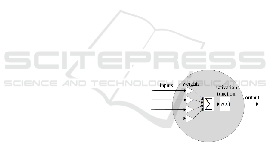
3.1.1 Neuron

A neuron can be mathematically described by its

activation, which represents the output. This

activation depends on the inputs of the neuron, the

weights of the inputs and the activation function.

Figure 1: Structure of a neuron.

The inputs 



are multiplied by their respective

weights 



and then summed up, so that the argument

 of the activation function  is calculated by:









∙



(1)

The weights  are the parameters that are gradually

adjusted and optimized during the training. They are

randomly initialized at the beginning.

Many different functions can be used for the

activation function. Karlik and Olgac (2011) compare

some common activation functions and analyse their

impact in the training performance. The activation

Development and Validation of Active Roll Control based on Actor-critic Neural Network Reinforcement Learning

function can be chosen separately for each layer or

even each single neuron in the artificial neural

network. The presented model in this article uses a

combination of three different functions: the

hyperbolic tangent shown in equation (2), a linear

function shown in equation (3) and the Rectified

Linear Unit shown in equation (4).











tanh

(2)











0,

(3)











 (4)

The function value of the activation function

represents the output of the neuron and is used either

as input to the neurons of the next network layer or as

output of the network.

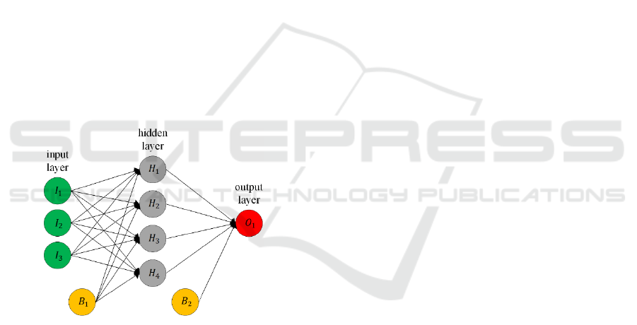
3.1.2 Topology

An artificial neural network consists of at least two

layers: the input and the output layer. For simple

learning problems, these two layers can be sufficient

to find an adequate solution. For more complex

systems, hidden layers are needed. If one or more

hidden layers are present, the term of deep learning is

applicable (Goodfellow et al., 2016).

Figure 2: Exemplary architecture of an artificial neural

network.

The input layer with the neurons  maintains the

values of the data sets used and thus the input of the

artificial neural network. The output layer with the

neurons maintains the output of the network. The

number of hidden layers with the neurons  is not

limited but is recommended to be kept as small as

possible to reduce its complexity.

In addition to the outputs of the previous layer,

every hidden layer and the output layer has a bias .

The bias is a constant value and can be parameterized

during training, since it is also multiplied with its

weights. It is necessary to calculate a constant offset,

which is independent of any inputs  e.g. for

compensating measuring noise.

The numerical relationship between the input and

output of the artificial neural network gives the

following:













∙

,













∙





,



(5)















∙

,





∙





,









(6)

With 



being the number of input neurons and 



being the number of neurons of the hidden layer.

If the inputs of a neuron consist only of the outputs

of the previous layer and the bias, it is referred to as a

feedforward network. If, on the other hand, the output

of the neuron is fed back as an input with a time delay,

a recurrent network is existent. This causes the output

of a neuron to become dependent on an output from

the previous time step. In this work, a fully connected

feedforward neural network is used.

3.1.3 Learning Rule

The learning rule is used to find suitable values for

the weights , with which the desired output is

achieved with a tolerable error. Equations (5) and (6)

show that the output is directly dependent on the

weights and the activation functions. An influence

during training only can be taken on the weights. The

basis of the most commonly used learning rules is the

Hebbian learning rule that says that a weight 

,

adjusted when neuron  and neuron  are active at the

same time (Hebb, 1949). The weight change ∆

,

dependent on the outputs of the respective neurons 



and 



and a fixed hyperparameter . It forms the

product of these three components, so the

mathematical expression for weight adjustment

becomes:

∆

,

∙



∙



(7)

The parameter  is the learning rate and an

elementary part of the training of an artificial neural

network. It decisively determines with which step

size the weights are adjusted. The learning rate can be

changed during training to ensure continuous learning

progress. However, an optimal learning rate cannot be

determined analytically due to the dependence on

randomness.

In this article a method with a gradient descent,

specifically backpropagation is presented. Therefore,

the squared error, also called loss , between the

SIMULTECH 2019 - 9th International Conference on Simulation and Modeling Methodologies, Technologies and Applications

desired output 



and the observed output 



, the

latter resulting from the random weight initialisation,

is calculated.

















(8)

The bisecting factor is used for simpler

differentiation. The loss represents the deviation from

the optimum the controller can achieve. So, the goal

of the artificial neural network is to minimize it in a

proper way. To use this error for the weight

adjustment the partial derivatives and thus the

gradient  is computed for every single weight. For

example, the modification of the weights between the

input and the first hidden layer is calculated as

follows:







,







,











∙









∙







,



(9)

With  being the summed-up inputs and  the output

of the respective neuron. Any connection between

layers can be computed analogously and thereby

every single weight can be adjusted separately. This

enables the possibility to propagate the summarized

error  back to every single weight and to customize

it accordingly. This gradient now is multiplied with

the learning rate  to get the weight change.

∆

,

∙





,



(10)

With advancing during the training, the loss

diminishes and thus the weight changes do. So, the

training always becomes more precise.

Because the gradient descent requires a given

output as a desired output 



to calculate the loss, it

is often used for supervised learning. This article

however shows how to use it with reinforcement

learning.

3.2 Reinforcement Learning

Reinforcement learning pursues the goal of assigning

inputs of the artificial neural network to certain

outputs in order to achieve a maximum reward

(Sutton and Barto, 2018). The artificial neural

network and the learning method, in the following

referred to as the agent, continuously interacts with

the system environment rather than with stored

training data sets as is the case in supervised or

unsupervised learning. The inputs of the artificial

neural network correspond to the states of the system

e.g. the roll angle and the outputs to the actions

carried out by the system e.g. the actuated torque. One

of the agent's responsibilities is determining the

desired nominal value 



. It does this without

having any information about which action to take in

which state or whether the last performed action was

right or wrong. Instead, it must find out through

appropriate training, which action leads to the highest

reward. This is calculated by the system environment

by a given reward function for the current state 



, the

associated executed action 



and the resulting state





and is to be selected so that the agent in the case

of the maximum value, performs the desired action.

The reward function should therefore always be set

up as a function of a desired reference state or action

and is calculated by:

1





²

(11)

With R being the reward and  the state or action to

be controlled with respect to the desired reference

state or action 



.This results in a maximum reward

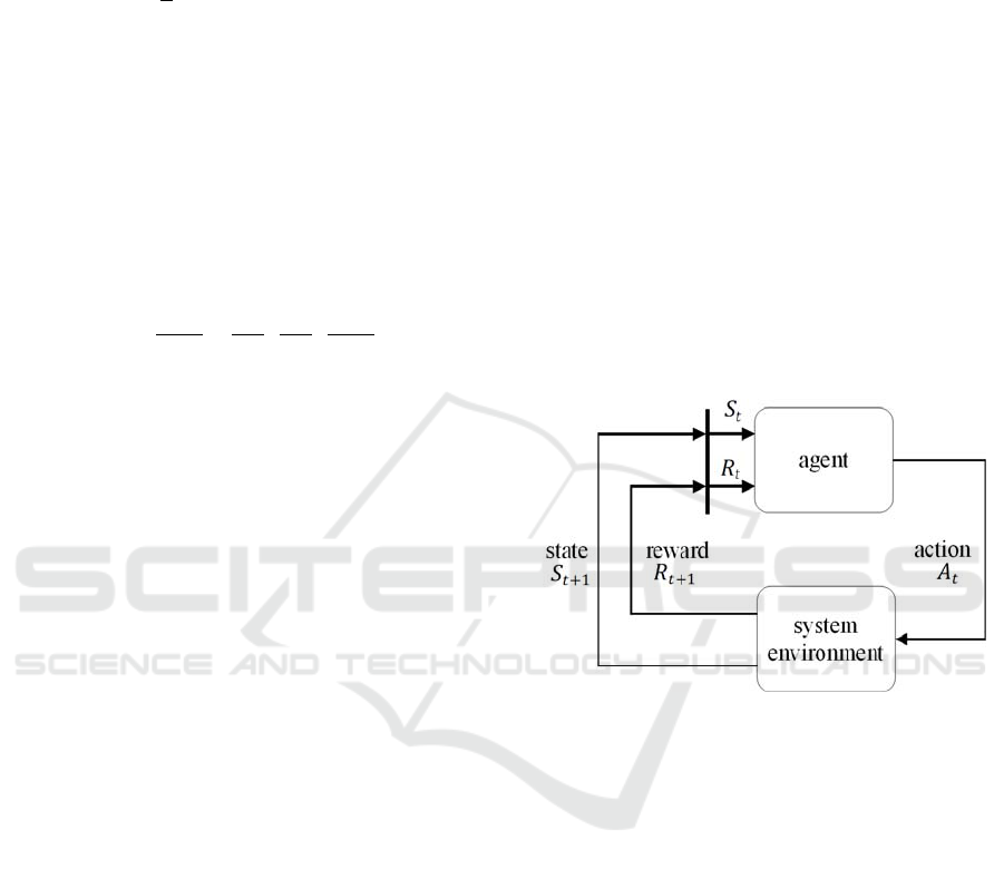
of one. Figure 3 shows the flow chart of

reinforcement learning.

Figure 3: Flow chart of reinforcement learning (Sutton and

Barto, 2018).

The agent receives the state  and a reward  from

the system environment in each time step  and

calculates an action  depending on the current level

of training. The assignment of the actions to the

respective states is summarized in the agent's

policy .















(12)

This policy will be adjusted during the training

through two simultaneous processes called

exploitation and exploration. In the case of

exploitation, the agent prefers already known and

executed actions that lead to a high reward. To be able

to get to know these actions and the underlying states

and thus incorporate them into its training data set, it

must react to states differently during exploration

than the previous training provides. This happens

through random variations of the already known

actions. The action selected by the agent may be

Development and Validation of Active Roll Control based on Actor-critic Neural Network Reinforcement Learning

numerically set with a randomly generated deviation

and thereby achieve a potentially higher reward. The

agent would therefore adapt its policy. Exploration

and time delayed reward are the two most important

characteristics that differentiate reinforcement

learning from other learning methods (Sutton and

Barto, 2018).

Due to this, it has the advantage that it can be

applied to interactive disciplines and to unknown,

dynamic environments and systems. While

supervised and unsupervised learning are limited to

learning data sets and extending to other data sets,

reinforcement learning can train follow-up states that

have been induced by the choice of the previous

action, thus involving a wide range of state-space.

3.2.1 Temporal Difference Learning

Temporal difference learning is a variant of value

approximation and is used by the Critic in the

developed model. Here, the agent adapts its policy not

only after a series of actions based on the return ,

which is simply the sum of successive rewards, but

continuously in each iteration step based on the

action-value function 





,



. This determines,

comparable to the return, the sum of successive

rewards. However, in this case it does not wait for the

following iteration steps to be performed and instead

uses the expected rewards from the current strategy.

This means that 





,



is always determined as a

function of the current policy and contains

approximated rather than real values. As a result, no

defined end of an episode is necessary, and the value

can be estimated continuously.



,



,

















,









(13)

The agent sets up a new prediction of the action-value

in each step. The basic idea of temporal difference

learning is to minimize the deviation between 

,

the current step and 

,

of the next step (Tesauro,

1995). This is done by adjusting the weights of the

artificial neural network by means of

backpropagation. The loss  to be minimized is then

defined as follows:











∙

,



,





.

(14)

In temporal difference learning, the policy  is

therefore not optimized directly, but rather its

evaluation in the form of the action-value 



3.2.2 Policy Gradient Method

An alternative to the value approximation or temporal

difference learning is the policy gradient method,

which is used by the Actor in the developed model.

The policy of the agent  is parameterized with the

weights  and a gradient method is used. Thus, a

policy  is trained, which assigns the actions directly

to the states by equation (12). Through selective

weight adjustment, the desired relationship between

states and actions can be achieved.

The gradient 









is approximated by the

current policy and the return 



and is used by

equation (10).







































,

















,







(15)

For a detailed explanation and derivation of the

method, the literature of Sutton et. al. is

recommended (Sutton and Barto, 2018).

Compared to temporal difference learning, a

policy is generated directly which maximizes the

approximated return 



depending on the gradient

instead of minimizing a deviation in the form of the

loss. Backpropagation can also be used for this

maximization of 



3.3 Actor-critic

A large majority of reinforcement learning methods

can be categorized as actor-only and critic-only

(Konda and Tsitsiklis, 2003). While the

approximation of the action value function is used for

the critic-only, the actor-only uses a policy gradient

approximation (Sutton et al., 1999).

A disadvantage of the policy gradient method is

that the estimation of the gradient 









has a high

variance and thus can lead to unwanted jumps in the

weight adjustment. In addition, each policy

adjustment creates a new gradient that is independent

of the previous one, which in turn prevents the

accumulation and consolidation of previous

information (Konda and Tsitsiklis, 2003). In the case

of a critic-only with a value approximation, on the

other hand, the policy is not optimized directly but via







,



. As a result, in principle good

approximations can be achieved, but there is no

guarantee that they will get close enough to their

optimum and achieve a sufficiently tolerable result.

The actor-critic model combines the advantages

and largely compensates the disadvantages of actor-

only and critic-only. Two separate artificial neural

networks are generated and trained, one each for the

actor and the critic. Together they form the agent.

The critic receives the state  and the reward 

from the system environment and the action  from

the actor. From these quantities, the action value  is

SIMULTECH 2019 - 9th International Conference on Simulation and Modeling Methodologies, Technologies and Applications

determined and the loss E optimized according to

equation (14). Then the critic transfers the

action-value to the actor, which maximizes it with the

policy gradient method. Since two successive actions

and states are required for temporal difference

learning, the states and actions are buffered and

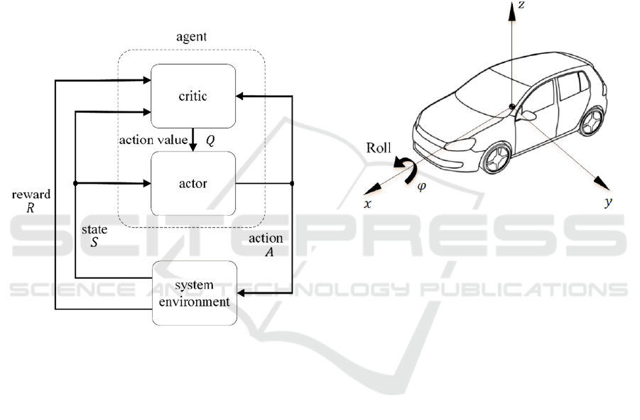
transferred in the next step. This results in the model

shown in figure 4.

For the adjustment of the critic the tuple









,



,



,



,





is necessary. The actor

determines its policy  using  and after completing

the training, it is the part of the model that represents

the neural controller, as it sends an action back to the

system environment depending on the state.

Figure 4: Flow chart of the used actor-critic model

(Szepesvári, 2009).

4 VEHICLE DYNAMICS

For the development of a neural controller, an

understanding of the dynamical system to be mapped

is not of great importance, since the neural controller

is supposed to independently recognize and apply the

respective structure. Nevertheless, the concepts of

rolling and stabilizing are explained shortly.

The term "roll" describes the rotation around the

body-fixed longitudinal axis, which is quantified by

the angle . This movement largely depends on the

lateral and vertical dynamics of the vehicle and is

shown in figure 5.

The stabilizer, which is the actuator of the active

roll control, is rotatably mounted on the vehicle body

and connected at both ends with the respective wheel

suspensions. With different deflection of the two

wheels, the levers experience differently large

deflections, which result in a twisting of the torsion

bar and thus in a corresponding torsional torque

(Schramm et al., 2018).

For an active influence by the stabilizer this is

mechanically separated in the middle and the

resulting free ends coupled via an actuator. This

actuator is performed in this work by an electric

motor. Instead of the passive torque generated by

torsion, the electro-mechanical actuator imprints a

torque which ensures a controlled influence on the

roll angle.

Figure 5: Roll angle of a motor vehicle (Schramm et al.,

2018).

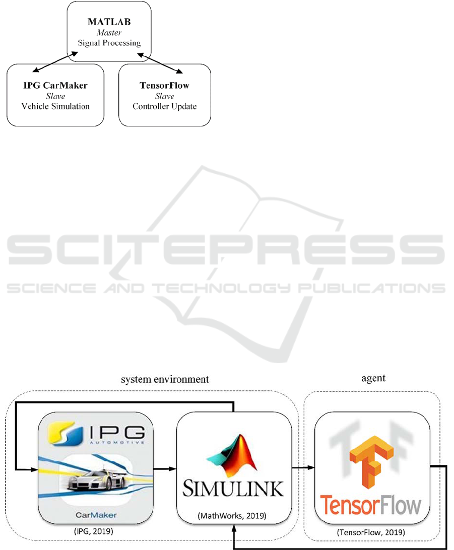
5 SIMULATION ENVIRONMENT

The training and validation of the controller is carried

out in simulation. The simulation environment

contains three software packages, each fulfilling

special requirements for the development process and

interacting in a master/slave communication shown in

figure 6. MATLAB is used as master. It guarantees

the communication and synchronization between the

different environments and can further be used for

any kind of signal processing. The training data is

generated by the software IPG CarMaker. It is used

for the task of a whole vehicle simulation in a virtual

environment. CarMaker offers an environment for

simulation and testing of whole vehicle systems under

realistic conditions. It provides driving conditions

dependent on different selection options such as the

used car or road. For the presented elaboration the

available Lexus RX400h, which is a Sport Utility

Vehicle (SUV) with one stabilizer per vehicle axle. A

detailed mathematical modeling is done within the

licensed software and is not directly visible to the

user.

Development and Validation of Active Roll Control based on Actor-critic Neural Network Reinforcement Learning

The track used is flat and has no slopes. The

vehicle can be controlled by providing physical

parameters via the interface in MATLAB/Simulink.

In this case the roll stabilization forces acting on the

car are manipulated.

Figure 6: Master/slave communication of the simulation

environment.

The driving conditions are transmitted to the

software MATLAB/Simulink in which the active roll

stabilization is realized. The results of this

stabilization are the mentioned stabilization forces in

dependence of the counter-torque 



. The

counter-torque required for roll stabilization

corresponds to the output of the artificial neural

network, which is constructed and trained with the

frame work and the open source libraries from

TensorFlow. The counter-torque 



 is calculated

by the neural network with respect to the states . In

this work the states are the the roll angle , the roll

velocity , the roll acceleration  and the lateral

acceleration 



. TensorFlow is included in the loop

during training since it offers the developer high

agility in building and altering the structure of

artificial neural networks. The driving states are

therefore sent via MATLAB/Simulink to the agent

formed by TensorFlow before the active roll

stabilization. After the agent has determined an

output in the form of the counter-roll torque 





as a function of the states, it sends this to

MATLAB/Simulink, where subsequently the

resulting roll stabilization forces acting on the vehicle

are transferred to IPG CarMaker. This feedback

message closes the simulation cycle. The data

exchange between MATLAB/Simulink and the

python based TensorFlow occurs through TCP/IP-

communication. The sample time of the simulation is





1 ms.

6 TRAINING

The training maneuvers represent the data available

during training and can be compared to the training

data set for supervised and unsupervised learning.

Depending on the learning problem, the methodology

of machine learning does not necessarily cover the

entire state space during training. Rather, the artificial

neural network is designed to develop and represent

an algorithm that provides satisfactory results in the

training data and is extra- and interpolatable over the

entire or most of the state space. The goal is to control

the roll angle . The desired reference angle in this

approach is 



0 which results in the reward

function with respect to equation (11):

1²

(16)

When choosing the training maneuvers, however,

care must be taken to provide the agent with data that

can be used for extrapolation and interpolation. For

suitable roll stabilization, accelerations and roll an-

Figure 7: Flow chart of simulation environment.

SIMULTECH 2019 - 9th International Conference on Simulation and Modeling Methodologies, Technologies and Applications

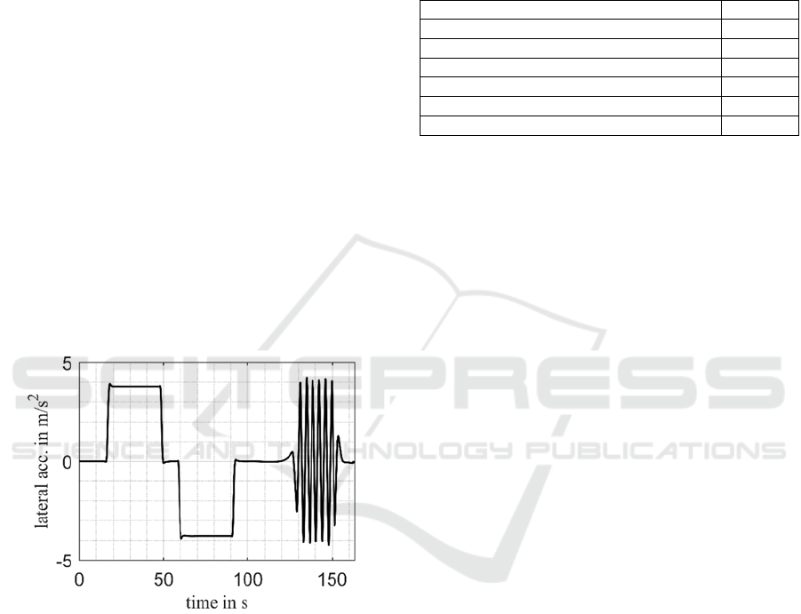
gles in both directions of the transverse axis must

therefore be available as input during training, so that

the neural controller can react differently to both

eventualities after completed training. For this reason,

the training maneuvers consist of stationary circular

drives according to ISO 4138 in both directions and a

slalom around pylons with a constant distance.

Stationary circular drives ensure that the agent

receives corresponding input variables over several

consecutive iteration steps, which require control and

contain lateral accelerations in one direction. This

allows the agent to train positive and negative

counter-torque separately in terms of time. Due to the

slalom ride, in which the lateral acceleration changes

periodically, the agent can train the steering angle

regarding variable driving dynamics. Straight

sections are inserted between the mentioned

maneuvers because the agent also has to learn to

deliver a torque of 



0 Nm (or an absolute small

torque) facing no (or relatively small) lateral

acceleration despite its randomly distributed start

weights. All training maneuvers are carried out with

the vehicle speed 70 km/h. The radius of

curvature of the circle runs is 100 m and the

pylon distance of the slalom ride 



36 m.

Figure 8: Lateral acceleration of the training maneuvers.

It should be noted here that the roll angle to be

controlled and the lateral acceleration have a dynamic

interaction, which causes the lateral acceleration to

change as a function of the set actuator torque during

the training. In addition, the three individual

maneuvers are repeated as often as desired and in

random order. The time-based arrangement of figure

8 thus only serves the compactness of the

representation and does not represent the training

course.

The preparation for training an artificial neural

network includes choosing several hyperparameters.

Calculation of optimal parameters is not readily

possible due to the highly interactive coupling and the

influence of the randomness that the agent requires

for its exploration in training. Training an artificial

neural network also means to adjust these parameters.

The finally used values for the most important

hyperparameters are shown in table 1.

Table 1: Most important used Hyperparameters.

Learnin

rate 0.0001

Number of neurons in first hidden la

100

Number of neurons in second hidden la

Variation standard deviation 2

Variation standard deviation decay 0.9999

Minimal variation 0.1

Reward deca

0.9

The importance of the learning rate  is

mentioned in chapter 3.1.3. The architecture contains

of two hidden layers with different number of

neurons. The variation ensures the exploration of the

agent needed for Reinforcement Learning and is

carried out by a Gaussian distribution with the

standard deviation of 2. The resulting value is then

added to the calculated output of the network to get

different responses than expected. Moreover, the

standard deviation of the variation is decreased over

the subsequent iteration steps of the training by its

decay. By doing this the agent is guaranteed to follow

his policy getting better throughout training period.

The standard deviation is multiplied with the decay in

every iteration step until getting to its minimum. The

Reward decay 



is used in equation (14) to lower the

influence of subsequent iteration steps compared to

the current iteration step.

The following presented results required 173

different training sessions while adjusting the

hyperparameters, the structure of the artificial neural

network and optimization algorithm. The session

leading to the final neural controller took about 20

million iteration steps and about 37 hours of

simulation time.

7 VALIDATION

Five different driving maneuvers are used to validate

the results. These consist of the training maneuvers

with varied radii, pylon distances and speeds and are

extended by the double lane change (ISO 3888-1). By

adding further driving maneuvers and varying the

traditional maneuvers, the interpolation and

extrapolability of the developed controller can be

evaluated. As a comparison, the passive roll stabilizer

is used. To assess the roll behaviour, the roll angle

Development and Validation of Active Roll Control based on Actor-critic Neural Network Reinforcement Learning

curve is compared in each case. For each maneuver

one case is selected to show its effect.

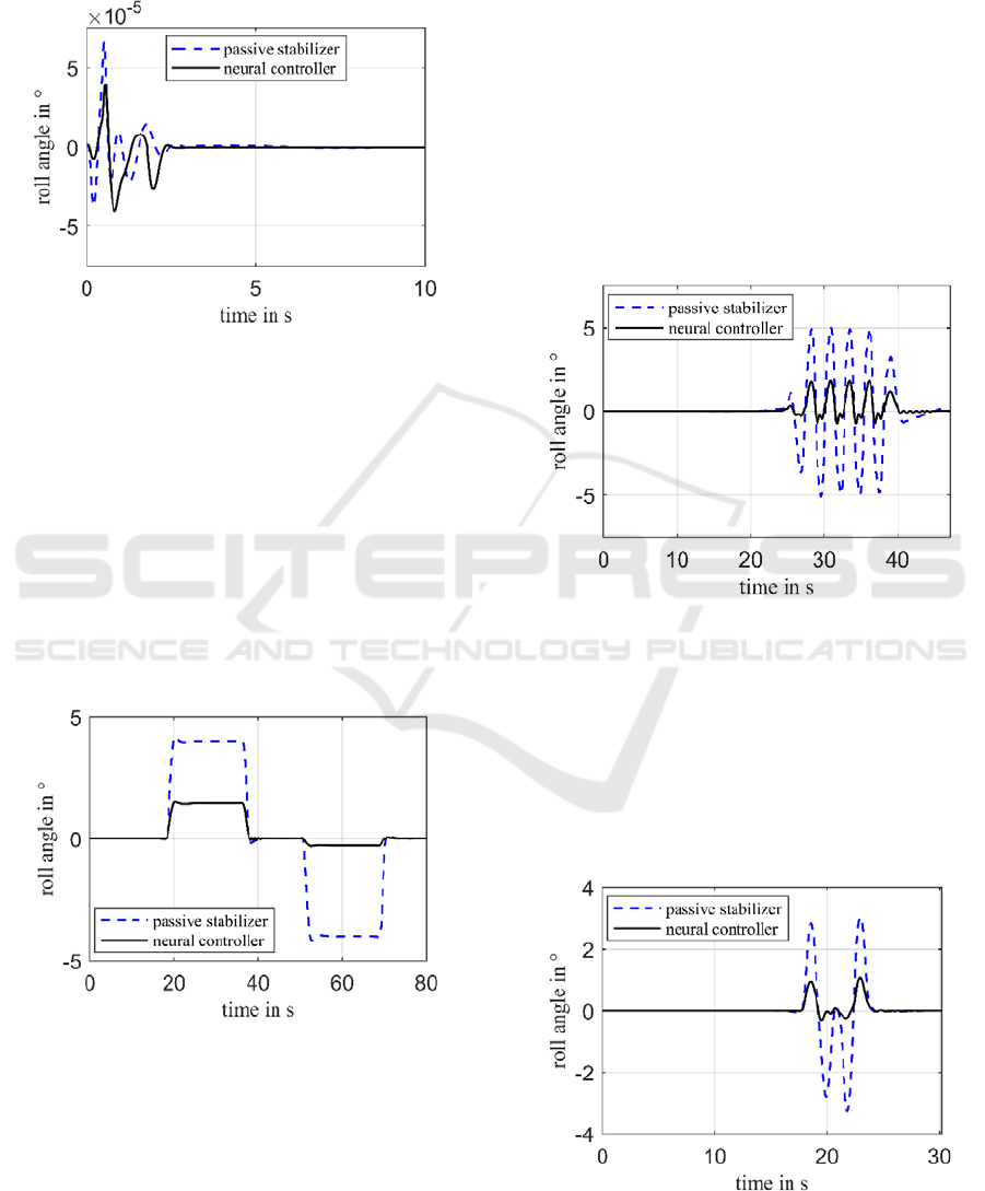
To validate the straight-ahead driving, this is

carried out at a speed of 50 km/h.

Figure 9: Straight-ahead driving at 50 km/h.

Figure 9 shows the roll angle for both the passive

stabilizer and the developed neural controller. Since

the vehicle has no lateral acceleration in a

straight-ahead drive without environmental

influences, the roll angle is constant 0 ° in the

case of a passive stabilizer. The deviance at the

beginning is neglectable and results from the

initialization of the vehicle with the simulation

environment. The developed neural controller shows

a similar behaviour.

For the stationary circuit (ISO 4138) the case with

50 km/h and 40 m is used.

Figure 10: Stationary circuit at 50 km/h and

40m.

The roll angle curve of the neural controller in

figure 10 works differently for negative and positive

lateral accelerations. Negative lateral accelerations

and roll angles are reduced more. A possible

explanation for this may be the random distribution

of the training maneuvers. In the test manager of IPG

CarMaker, driving maneuvers can be inserted,

duplicated as often as desired and then mixed. There

was a significantly higher number of the training

maneuvers for the training than was possible during

the training period. As a result, there is a possibility

that the mixture during training has significantly more

right-handed than left-handed curves, which can lead

to the observed differential behaviour. With the

neural controller, the roll angle in the left-handed

curve can be reduced from 



4 ° to 





1.47 °, resulting in a 63.25% reduction. In the

right-handed curve, a roll angle of 



0.28 ° and

thus a 93% reduction is achieved.

The validation is shown exemplary at 

50 km/h and a pylon distance of 



18 m.

Figure 11: Slalom at 50 km/h and 



18 m.

The result of the slalom ride reflects the previous

findings. The different control behaviour for negative

and positive lateral accelerations can be seen. Since

there are no irregularities in the six different slalom

runs with different speeds and pylon distances, it can

be concluded that the control behaviour of the neural

controller for slalom driving is extra- and

interpolatable.

Figure 12: Double lane change at 60 km/h.

SIMULTECH 2019 - 9th International Conference on Simulation and Modeling Methodologies, Technologies and Applications

The double lane change (ISO 3888-1) is a pure

validation maneuver and thus evokes a driving

dynamic that was not explicitly trained by the agent.

However, this driving dynamic is comparable to that

of a slalom, so that similar results can be expected. It

is validated exemplary at 60 km/h.

As expected, the control behaviour of the neural

controller is very similar to that of slalom driving. It

shows that the control behaviour can also be

extrapolated to other maneuvers and driving

situations.

8 CONCLUSIONS

In the context of this work an active roll control with

an artificial neural network based on an actor-critic

reinforcement learning method has been successfully

realized. The neural controller was realized with the

TensorFlow libraries in a Python script and combined

with the simulation model of the entire vehicle and

the active roll stabilization contained therein via a

TCP/IP interface.

A guaranteed calculation of the torque to be set in

a fixed time interval and a time limit of the waiting

time of the TCP/IP interface created a real-time

control. If, in the defined waiting time, the actuator

does not receive any action from the neural network,

the torque is set from the previous time step. The

developed neural controller is able, at any time, to

stably reduce the roll angle caused by the centrifugal

force of the vehicle body by means of an actuator. The

functionality of the controller is thus given.

The results show that the developed controller

produces a rather uneven roll behaviour for both

directions of the steering angle in comparison to

established, conventional controllers. However, it has

been proven that roll stabilization by artificial neural

networks is possible and that the developed model is

able to replace conventional controllers. If the

knowledge gained in this work continues to be

applied to the model and extended with small and

precise optimizations, a neural controller with

symmetric behaviour can be trained for lateral

acceleration in both directions. Since the field of

machine learning works with very complex contexts

and is strongly randomized, this is a matter of time.

Basically, in 100 training runs with identical

hyperparameters, 100 different results can be

achieved, the extent of which is far from expedient.

Nonetheless, it has been shown that the neural

network used can provide a controller with tolerable

results. A fixed reproducibility of this result is not

given by the immense influence of randomness, but

due to the stochastics also better results are possible.

Due to its structure, the agent is able to adjust its

weights so that, for positive lateral accelerations, an

at least equal reduction of the roll angle is achieved,

as for negative transverse accelerations.

Further works will investigate the influence and

possible improvements by applying a regularization

on the weight adjustment to ensure the minimal

optimal weights and symmetric behaviour for

positive and negative lateral accelerations.

REFERENCES

Boada, M., Boada, B., Gauchia Babe, A. Calvo, J. and Diaz,

V., 2009. Active roll control using reinforcement

learning for a single unit heavy vehicle. In International

Journal of Heavy Vehicle Systems, 16(4), pp. 412-430.

Fu, Z.-J., Li, B., Ning, X.-B., Xie and W.-D., 2017. Online

Adaptive Optimal Control of Vehicle Active

Suspension Systems Using Single-Network

Approximate Dynamic Programming. In Mathematical

Problems in Engineering.

Goodfellow, I., Bengio, Y. and Courville, A., 2016. Deep

Learning, The MIT Press. London.

Hebb, D., 1949. The Organization of Behavior, John Wiley

& Sons, Inc. New York.

IPG, 2019. IPG Automotive’s Official Website. [online]

Available at https://ipg-automotive.com/ [Accessed

09 Feb. 2019].

Karlik, B. and Olgac, V., 2011. Performance Analysis of

Various Activation Functions in Generalized MLP

Architectures of Neural Networks. In International

Journal of Artificial Intelligence and Expert Systems

(IJAE), 1(4), pp. 111-122.

Konda, V. and Tsitsiklis, J., 2003. Actor-Critic Algorithms.

In SIAM Journal on Control and Optimization, 42(4),

pp. 1143-1166.

Li, H., Guo, C. and Jin, H., 2005. Design of Adaptive

Inverse Mode Wavelet Neural Network Controller of

Fin Stabilizer. In International Conference on Neural

Networks and Brain, 2005, 3, pp. 1745-1748.

MathWorks, 2019. MathWorks’ Official Website. [online]

Available at https://de.mathworks.com/ [Accessed 09

Feb. 2019].

Rosenblatt, F., 1958. The Perceptron: A probabilistic model

for information storage and organization in the brain. In

Psychological Review, 65(6), pp. 386-408.

Schramm, D., Hiller, M. and Bardini, R., 2018. Vehicle

Dynamics – Modeling and Simulation, Springer.

Edition.

Sieberg, P., Reicherts, S. and Schramm, D., 2018.

Nichtlineare modellbasierte prädiktive Regelung zur

aktiven Wankstabilisierung von Personenkraftwagen.

In 4

IFToMM D-A-CH Konferenz 2018.

Sutton, R. and Barto, A., 2018. Reinforcement Learning: An

Introduction, The MIT Press. London, 2

edition.

Development and Validation of Active Roll Control based on Actor-critic Neural Network Reinforcement Learning

Sutton, R., McAllester, D., Singh, S. and Mansour, Y.,

1999. Policy Gradient Methods for Reinforcement

Learning with Function Approximation. In NIPS'99 -

Proceedings of the 12th International Conference on

Neural Information Processing Systems, pp.

1057-1063.

Szepesvári, C., 2009. Algorithms for Reinforcement

Learning, Morgan & Claypool Publishers.

TensorFlow, 2019. TensorFlow’s Official Website. [online]

Available at https://www.tensorflow.org/ [Accessed

09 Feb. 2019].

Tesauro, G., 1995. Temporal Difference Learning and TD-

Gammon. In Communications of the ACM, 38(3), pp.

58-68.

SIMULTECH 2019 - 9th International Conference on Simulation and Modeling Methodologies, Technologies and Applications