Stochastic Models of Non-stationary Time Series of the Average Daily

Heat Index

Nina Kargapolova

Laboratory of Stochastic Problems, Institute of Computational Mathematics and Mathematical Geophysics SB RAS,

Pr. Ak. Lavrent’eva 6, Novosibirsk, Russia

Department of Mathematics and Mechanics, Novosibirsk State University, Novosibirsk, Russia

Keywords: Stochastic Simulation, Non-stationary Random Process, Heat Index, Air Temperature, Relative Humidity,

Model Validation.

Abstract: In this paper two numerical stochastic models of time series of the average daily heat index are considered.

In the first model, time series of the heat index are constructed as a function of simulated joint nonstationary

time series of air temperature and relative humidity. The second model is constructed under the assumption

that time series of the heat index are non-stationary non-Gaussian random processes. Data from real

observations at weather stations were used for estimating models’ parameters. On the basis of the simulated

trajectories, some statistical properties of rare meteorological events, like long periods of time with high heat

index, are studied.

1 INTRODUCTION

It is known that of all the effects of the environment

on human beings, one of the most significant for the

human health and well-being are the factors

determining the thermal state of a person. With

adverse combinations of these factors, there is a threat

of hypothermia or overheating of a body (Kobisheva

et al., 2008; McGregor et al., 2015; Zare et al., 2018).

Different bioclimatic indices (heat / cold stress index,

heat index, weather severity index, etc.) are used to

assess the combined heat effects on the human body

of high temperature and relative humidity, cold

humid air and wind speed, as well as other

meteorological processes.

At present, to study the properties of the time

series of bioclimatic indices two approaches are

mainly used. In the framework of the statistical

approach, data from real observations are analyzed,

see, for example, (Kershaw and Millward, 2012;

Revich and Shaposhnikov, 2018; Shartova et al.,

2018). The second approach is a dynamical one – it is

based on the use of hydrodynamic models of

atmospheric processes (Gosling et al., 2009; Ohashi

et al., 2014).

https://orcid.org/0000-0002-1598-7675

In 2018, the author of the paper together with

colleagues at the Institute of Computational

Mathematics and Mathematical Geophysics SB RAS

(Novosibirsk, Russia) and the Voeikov Main

Geophysical Observatory (St. Petersburg, Russia)

began the development of a stochastic approach to

studying and simulation of the time series of

bioclimatic indices. For short time intervals (about

10–12 days), models of high-resolution time series of

the heat index and the enthalpy of humid air were

constructed and validated. These models take into

account the daily variations of the real weather

processes (Kargapolova et al., 2019).

The objective of this paper is to propose such a

stochastic model of time series of the average daily

heat index (ADHI) on a long intervals that would take

into account the influence of a seasonal variation of

air temperature and relative humidity on the time

series of the ADHI. In this paper two stochastic

models are considered. It is shown that the model

based on simulation of the joint time series of air

temperature and relative humidity does not reproduce

properties of the ADHI time series as good as it

reproduces properties of the high-resolution time

series of the heat index. In contrast, a model based on

simulation of the ADHI time series using the inverse

Kargapolova, N.

Stochastic Models of Non-stationary Time Series of the Average Daily Heat Index.

DOI: 10.5220/0007788502090215

In Proceedings of the 9th International Conference on Simulation and Modeling Methodologies, Technologies and Applications (SIMULTECH 2019), pages 209-215

ISBN: 978-989-758-381-0

209

distribution function method describes the real

process precise enough.

2 THE HEAT INDEX

To describe the influence of high air temperature and

relative humidity on a human being the so-called

“heat index” is frequently used (Steadman,1979;

Steadman, 1984). The overview and comparison of

existing approaches to the definition of this index is

provided in (Anderson et al., 2013). In this paper, the

average daily heat index

is defined using the

approach, proposed in (Schoen, 2005):

 





0 0801 14

0 03755

1 0799 1

237 3 17 27

17 27 237 3

HI T . e e ,

. . T

D , lnH,

. . T





  

  



(1)

where

and

are the average daily air

temperature and relative humidity, respectively,

is dew point temperature. Here unit of measurement

of air temperature is a Celsius degree, and relative

humidity is measured in fractions of unity; the heat is

supposed to be dimensionless. It should be noted that

the heat index is not measured at weather stations, but

it could be calculated using the above-given formulas

based on the observed values of air temperature and

relative humidity.

Let

 

12 N

HI HI ,HI , ,HI

denote time series

of the average daily heat index (ADHI) on a

N 

day

interval.

3 THE TH-MODEL

Since the heat index is a function of air temperature

and relative humidity, a natural approach to the

simulation of its time series is to simulate the joint

time series of air temperature and relative humidity

and then to calculate values of the heat index. Such an

approach was proposed and validated in

(Kargapolova et al., 2019) for the simulation of high-

resolution time series of the heat index at short time

intervals. The model proposed therein is based on the

model of periodically correlated joint time series of

air temperature and relative humidity detailed in

(Kargapolova et al., 2018).

Let us apply the approach described to the

simulation of time series of the ADHI at long time

intervals. Statistical analysis of real meteorological

data reveals that the joint time series

 

1 2 1 2NN

T,H T ,T , ,T ,H ,H , ,H

of the

average daily air temperature and relative humidity

long time intervals are non-stationary.

One-dimensional distributions and a correlation

structure of the joint time series of air temperature and

relative humidity are used as the model input

parameters.

In order to construct a stochastic model, the use of

sample one-dimensional distributions is not

reasonable, since the sample distributions do not have

any tails, and therefore do not allow one to estimate

the probability of occurrence of extreme values of the

heat index. In this connection, it is necessary to

approximate the sample distributions densities by

certain analytic densities, which, on the one hand, do

not greatly alter the form of a sample distribution and

its moments, and on the other – possess tails.

It should be noted that for approximation of the

empirical one-dimensional distribution

 

of the

average daily temperature, the Gaussian distribution

is often used (Ogorodnikov, 2013; Richardson, 1981;

Richardson and Wright, 1984). However, the

numerical experiments have shown that if, despite an

increase in the complexity of simulation, one

approximates the temperature distribution with a

mixture

 

exp

1 exp ,

0 1, 1,N

















  











  





  

(2)

of the two Gaussian distributions, the quality of the

model being significantly improved. In this paper, the

parameters

1 1 2 2

, , , , , 1,N

k k k k k

a b a b k





were

chosen using the algorithm, proposed in (Marchenko

and Minakova, 1980). This algorithm makes possible

to choose such parameters of the density (2) (and the

corresponding CDF

 

) that mathematical

expectation, variance and skewness of a random

variable with the density

 

should be equal to

the corresponding sample characteristics, and the

function

 

minimizes the Pearson functional

that describes the difference between

 

and

 

For approximation of one-dimensional

distributions of the average daily relative humidity

SIMULTECH 2019 - 9th International Conference on Simulation and Modeling Methodologies, Technologies and Applications

210

densities that are mixtures

 

of the two Beta-

distributions (with the corresponding CDF

 

)

are used.

In this paper, to construct a model of the time

series

 

T,H

(and hence a model of time series

) the

22NN

sample correlation matrix

T TH

HT H









(3)

is used. Here

are the sample autocorrelation

matrices of air temperature and relative humidity,

respectively, and

TH HT

are the sample cross-

correlation matrices of these two weather elements.

For the simulation of

 

T,H

with given one-

dimensional distributions (1) and a given correlation

matrix (3), the method of inverse distribution function

was used (Ogorodnikov and Prigarin, 1996). In the

framework of this method, simulating the sequence

comes down to an algorithm with four steps:

Step 1. Calculation of the matrix



that is a

correlation matrix of an auxiliary standard Gaussian

process

 

T',H'

. The element

 

i, jr



, 1,2i j N

of the matrix



is the solution to the equation

 

i, j

i, , ,,j

F x F y x y d

G x i N

B x i

xdy









 









  















where

 

i, jr

is an element of the matrix

corresponding to

 

i, jr



, the function

 

,, i, jxyr





is a distribution density of a bivariate Gaussian vector

with zero mean, variance equal to

and the

correlation coefficient

 

i, jr



between components

number

and

 



is a CDF of a standard

normal distribution.

Step 2. Simulation of the standard Gaussian

sequence

 

T',H'

with the correlation matrix



Step 3. Transformation of

 

T',H'

into

 

T,H

















, 1, ,

, 1,

i i i

j j j

T G T i N

H B H j N





  



  

Step 4. Calculation of

using its definition (1)

given in the previous section.

If the matrix



, obtained at the first step, is not

positive definite, it must be regularized. Several

methods of regularization are described in

(Ogorodnikov and Prigarin, 1996). In this paper, the

method of regularization based on substitution of

negative eigenvalues of the matrix

with small

positive numbers was used. At the second step, the

simulation of the standard Gaussian sequence

 

T',H'

with the correlation matrix

could be

done using the Cholesky or the spectral

decomposition of the matrix

(Ogorodnikov and

Prigarin, 1996). The latter is used here. Steps 2-4 are

repeated as many times as many trajectories are

required.

Any stochastic model has to be verified before one

starts to use simulated trajectories to study properties

of a simulated process. For model verification, it is

necessary to compare simulated and real data based

estimations of such characteristics, which, on the one

hand, are reliably estimated by real data, and on the

other hand are not input parameters of the model.

In this paper, the long-term observations data

from weather stations located in different climatic

zones were used for verification. Although all

examples in this paper are given only for the stations

in the cities of Sochi (the Black Sea region, years of

observation: 1993-2015) and Astrakhan (the Caspian

Sea region, years of observation: 1966-2000), all the

conclusions are valid for all considered weather

stations.

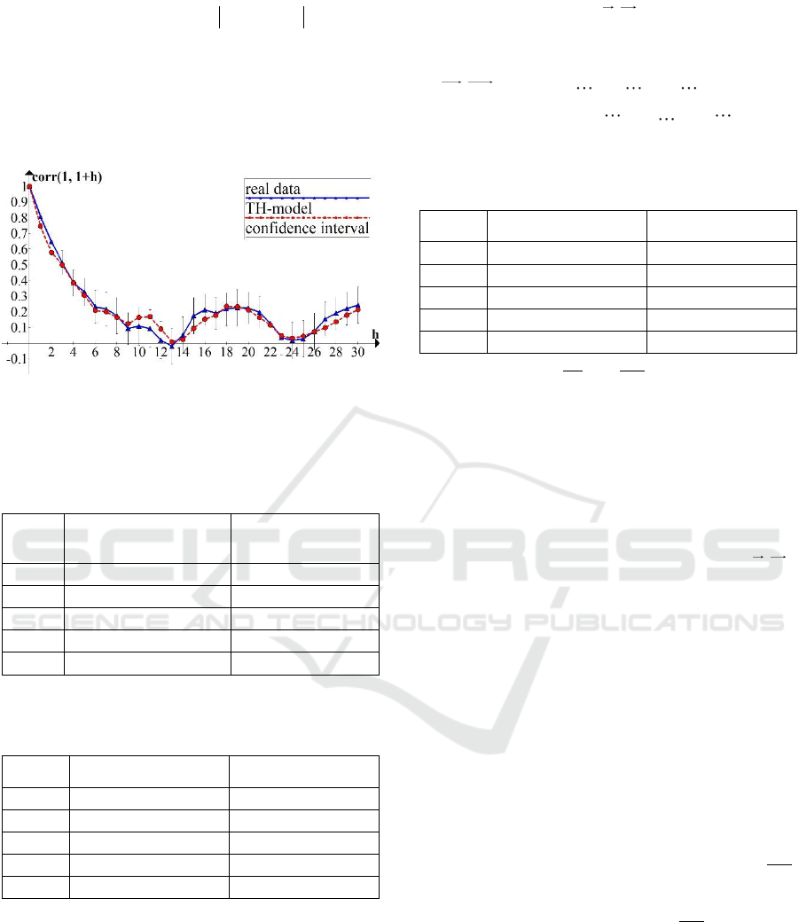
The correlation coefficients

 

corr HI HI

the ADHI time series are not input parameters of the

TH-model, so they could be used for the verification

of this model. Figure 1 shows the correlation

coefficients

 

corr HI HI



, estimated with real

data (with



confidence interval) and with the

trajectories obtained with the TH-model. Numerical

experiments show that for all considered weather

stations and time intervals, the absolute difference of

correlation coefficients estimated with real and

simulated data does not exceed



. Hereinafter,



is a statistical estimate of the standard deviation of the

characteristic under consideration when estimating

with real data. Thus, the TH-model well reproduces

the correlation structure of time series of the ADHI.

As a matter of fact, other properties of real time

series of the ADHI are either not reproduced or poorly

reproduced by the TH-model. As an illustration,

Tables 1-3 show estimations of the average number

 

AN lev

of the days in a considered time-interval

with the ADHI above given level

lev

and estimations

Stochastic Models of Non-stationary Time Series of the Average Daily Heat Index

211

of the probability

 

1ii

p l P HI HI l



  

of a

rapid change in the heat index. Simulated data bases

estimations are given with significant digits only.

This means that the TH-model, despite its soundness

and applicability in cases of the high-resolution time

series, should not be used for the simulation of the

time series of the ADHI.

Figure 1: Correlation coefficients

 

corr HI HI



Astrakhan. July, 1-31.

Table 1: Estimations of

 

AN lev

. Astrakhan. August, 1-

31.

lev

Real data,

 

3AN lev





TH-model

28.206



1.630

27.193

21.088



2.819

14.463

10.441



0.887

1.032

2.853



1.586

0.007

0.500



0.640

0.000

Table 2: Estimations of the probability

 

. Sochi. June,

1-30.

Real data,

 

3pl





TH-model

0.585



0.063

0.577

0.304



0.037

0.275

0.150



0.055

0.111

0.078



0.039

0.040

0.039



0.054

0.013

The most probable reason for the invalidity of the

TH-model is related to the fact that the heat index is

a nonlinear function of air temperature and relative

humidity. It leads to the significant difference

between the ADHI calculated with the average daily

temperature and relative humidity (as in the TH-

model) and the ADHI calculated as an average of the

values of the heat index calculated with real

meteorological high-resolution data. To avoid this

problem, instead of the

 

T,H

one should simulate

the high-resolution time series

 

1 2 1

1 1 1

T ,T , ,T , ,T ,, ,T ,

T ,H ,

H , ,H , ,H , ,H











Table 3: Estimations of the probability

 

. Astrakhan.

June, 1-30.

Real data,

 

3pl





TH-model

0.685



0.047

0.588

0.422



0.055

0.283

0.223



0.050

0.113

0.106



0.040

0.038

0.055



0.029

0.011

where

T ,H , k ,n, i ,N

are temperature and

relative humidity measured

times per day in a day

number

, respectively, then calculate the high-

resolution time series of the heat index and average

them to obtain the ADHI. It should be noted that this

approach to the simulation is time-consuming (for

instance, one has to solve

times more equations to

define the correlation matrix of an auxiliary Gaussian

process than in case of the simulation of the

 

T,H

time series).

4 THE HI-MODEL

In this section, another approach to the simulation of

the time series of the average daily heat index is

considered. In the framework of this approach

(denoted as the HI-model), at the first step, a sample

of real time series of the ADHI is formed using the

long-term observation data about the average daily

temperature and relative humidity. Then sample

histograms are approximated with some one-

dimensional distribution densities

 

, 1,

n x k N

and a sample

NN

correlation matrix

estimated. In this paper,

 

, 1,

n x k N

is a mixture

of the two Gaussian distributions. Parameters of these

mixtures were chosen just as parameters of the

densities

 

. To construct a completely

parametric stochastic model of the time series, it is

necessary to approximate the sample correlation

function with some analytic parametric function (like

was done with one-dimensional distributions). Such

SIMULTECH 2019 - 9th International Conference on Simulation and Modeling Methodologies, Technologies and Applications

212

an approximation is in the course of development.

The last step is the simulation of trajectories of the

ADHI with the given densities

 

, 1,

n x k N

and

the correlation matrix

using the method of

inverse distribution function (in a similar way to steps

1-3 in the TH-model).

Results of verification of the HI-model are

provided below.

Tables 4 and 5 show the estimations of the

average number

 

AN lev

, defined in the previous

section. It is clearly seen that the HI-model well

reproduces this characteristic of the ADHI time series

both for harmless levels

lev

and for dangerous levels

(the heat index between 32 and 41 is the extreme

caution, between 41 and 54 is danger, above 54 is the

extreme danger).

Table 4: Estimations of

 

AN lev

. Astrakhan. August, 1-

31.

lev

Real data,

 

AN lev





HI-model

28.206



0.451

28.120

21.088



0.857

21.053

10.441



0.946

10.323

2.853



0.529

2.758

0.500



0.213

0.566

0.118



0.085

0.138

0.029



0.048

0.056

0.000



0.011

0.004

Table 5: Estimations of

 

AN lev

. Sochi. July, 1-31.

lev

Real data,

 

AN lev





HI-model

30.565



0.234

30.515

27.652



0.696

27.893

19.435



1.323

19.753

10.261



1.248

9.960

3.391



0.768

3.564

1.044



0.379

0.952

0.130



0.115

0.108

0.000



0.035

0.012

0.000



0.010

0.001

Another characteristic that was used both for the

verification of the HI-model and for the study of the

heat index time series properties was the probability

 

.pl

Tables 6 and 7 show the estimations of

 

based on real data and simulated trajectories. For all

the considered weather stations and time intervals, the

absolute difference of

 

estimated on real and

simulated data does not exceed



. This means that

this characteristic is well reproduced by the HI-

model.

The verification of the HI-model has shown that

this model with high accuracy reproduces many of the

statistical characteristics of real ADHI time series.

Accordingly, it is possible to use the HI-model to

study those properties of the time series that cannot

be studied using real data. Among other things, it is

possible to investigate an impact of an increase in the

average air temperature on the duration of periods

with the extremely high ADHI, on probability of the

occurrence of dangerous values of the ADHI and

other properties of adverse weather phenomena.

Below the results of one of the numerical experiments

conducted using the HI-model are given.

Table 6: Estimations of the probability

 

. Sochi. June

1-30.

Real data,

 





HI-model

0.585



0.021

0.638

0.304



0.022

0.360

0.150



0.018

0.183

0.078



0.013

0.084

0.039



0.008

0.035

0.021



0.005

0.014

0.011



0.003

0.005

0.006



0.002

0.000



0.001

0.000



0.001

0.000

The main idea of the experiment was to increase

the average daily temperature on condition that

relative humidity does not change, to estimate the

parameters of the distributions used in the HI-model

using the simulated temperature data, real relative

humidity data and real correlation coefficients, to

simulate the time series of the ADHI and to access an

average number

 

AN lev

of the days with the ADHI

above level

lev

. Simulation of air temperature non-

stationary time series was based on the model

proposed in (Kargapolova, 2018). Figure 2 shows the

results of this experiment for the four cases: when the

real average daily temperature was used and when the

average daily temperature was increased by

0.1 , 0.5 , 1.0

o o o

C C C

, respectively. The analysis

shows that for

32lev 

(recall that it is the extreme

caution level) the number

 

AN lev

increases by

Stochastic Models of Non-stationary Time Series of the Average Daily Heat Index

213

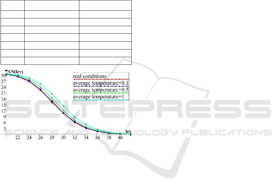
40 50%

depending on a weather station

considered. For level

lev

above

values of the

 

AN lev

almost double. This means that

1.0

rise

in the average air temperature causes a hefty increase

of days when people must be careful being outside. In

this numerical experiment the simplest warming

scenario was used.

Table 7: Estimations of the probability

 

. Astrakhan.

June 1-30.

Real data,

 





HI-model

0.685



0.016

0.698

0.223



0.017

0.255

0.055



0.010

0.069

0.018



0.004

0.015

0.007



0.002

0.003



0.001



0.001

0.000

Figure 2: Average number

 

AN lev

of days with the

ADHI above level

lev

. Astrakhan. July, 1-31.

For a detailed study of the climate change

influence it is necessary to use more complex

scenarios. For example, dependence between

changing temperature and relative humidity is meant

to be taken into account. Study the possible

alternation of the ADHI using complex climate

change scenarios and stochastic models calls for

further investigations.

5 CONCLUSIONS

In this paper, it is shown that the TH-model used to

simulate high-resolution time series of the heat index

cannot be used to simulate the ADHI series. Another

approach (the HI-model) to the simulation of these

time series is proposed. The results of verification of

the HI-model and an example of its application for

studying the ADHI properties, which cannot be

studied from real data, are given.

In the future, it is intended to use the model

constructed for solving a number of bioclimatological

problems related to development of proper heat-/cold

waves prediction systems and long-range forecasting

of the climate regime alteration. To solve these

problems, it is necessary to turn the proposed model

into a fully parametric one and to add a capability to

simulate conditional time series.

ACKNOWLEDGEMENTS

This work was partly financially supported by the

Russian Foundation for Basic Research (grant No 18-

01-00149-a), Russian Foundation for Basic Research

and Government of Novosibirsk region (grant No 19-

41-543001-r_mol_a).

REFERENCES

Anderson, G.B., Bell, M.L., Peng, R.D., 2013. Methods to

calculate the heat index as an exposure metric in

environmental health research. In Env. Health

Perspect., Vol. 121, No 10. P. 1111-1119.

Gosling, S.N., McGregor, G.R., Lowe, J.A., 2009. Climate

change and heat-related mortality in six cities. Part 2:

climate model evaluation and projected impacts from

changes in the mean and variability of temperature with

climate change. In Int J Biometeorol., Vol.53, No 1. P.

31-51.

Kargapolova, N. A., 2018. Monte Carlo Simulation of Non-

stationary Air Temperature Time-Series. In Proc. of 8th

Int. Conf. on Simulation and Modeling Methodologies,

Technologies and Applications “SIMULTECH-2018”.

P. 323-329.

Kargapolova, N. A., Khlebnikova, E. I., Ogorodnikov, V.

A., 2018. Monte Carlo simulation of the joint non-

Gaussian periodically correlated time-series of air

temperature and relative humidity. In Statistical papers,

Vol. 59. P.1471-1481.

Kargapolova, N. A., Khlebnikova, E. I., Ogorodnikov, V.

A., 2019. Numerical study of properties of air heat

content indicators based on the stochastic model of the

meteorological processes. In Russ. J. Num. Anal. Math.

Modelling, Vol. 34, No 2. P. 95-104.

Kershaw, S.E., Millward, A.A., 2012. A spatio-temporal

index for heat vulnerability assessment. In Environ.

Monit. Assess., Vol. 184. P. 7329-7342.

Kobisheva, N.V., Stadnik, V.V., Klueva, M.V., Pigoltsina,

G.B., Akentieva, E.M., Galuk, L.P., Razova, E.N.,

Semenov, U.A., 2008. Guidance on specialized

climatological service of the economy. Asterion. St.

Petersburg. (in Russian)

SIMULTECH 2019 - 9th International Conference on Simulation and Modeling Methodologies, Technologies and Applications

214

Marchenko, A.S., Minakova, L.A., 1980. Probabilistic

model of air temperature time-series. In Meteorology

and Hydrology, No 9. P. 39-47. (in Russian)

McGregor, G.R., Bessemoulin, P., Ebi, K., Menne, B.,

2015. Heatwaves and Health: Guidance on Warning-

System Development. WMO &WHO.

Ogorodnikov, V.A., 2013. Stochastic models of

meteorological processes: Teaching aid. NSU.

Novosibirsk.

Ogorodnikov, V.A., Prigarin, S.M., 1996. Numerical

Modelling of Random Processes and Fields:

Algorithms and Applications, VSP. Utrecht.

Ohashi, Y., Kikegawa, Y., Ihara, T., Sugiyama. N., 2014.

Numerical Simulations of Outdoor Heat Stress Index

and Heat Disorder Risk in the 23 Wards of Tokyo. In J.

Appl. Meteor. Climatol., Vol. 53. P. 583-597.

Revich, B., Shaposhnikov, D.A., 2016. Cold waves in the

southern cities of the European part of Russia and

premature mortality of the population. In Problems of

forecasting, No 2. P. 125-131. (in Russian)

Richardson, C. W., 1981. Stochastic simulation of daily

precipitation, temperature and solar radiation. In Water

Resour. Res., Vol. 17. P. 182-190.

Richardson, C. W., Wright, D.A., 1984. WGEN: A Model

for Generating Daily Weather Variables. U. S.

Department of Agriculture, Agricultural Research

Service.

Schoen, C., 2005. A new empirical model of the

temperature– humidity index. In J Appl Meteorol., Vol

44. P. 1413-1420.

Shartova, N., Shaposhnikov, D., Konstantinov, P., Revich,

B., 2018. Cardiovascular mortality during heat waves

in temperate climate: an association with bioclimatic

indices. In Int. J. of Environmental Health Research,

Vol. 28, No. 5. P. 522-534.

Steadman, R.G., 1979. The Assessment of Sultriness, Part

I: A Temperature-Humidity Index Based on Human

Physiology and Clothing Science. In J. Appl. Meteor.,

Vol. 18. P.861-873.

Steadman, R.G., 1984. A universal scale of apparent

temperature. In J Climate Appl Meteorol., Vol. 23. P.

1674-1687.

Zare, S., Hasheminejad, N., Shirvan, H.E., Hemmatjo, R.,

Sarebanzadeh, K., Ahmadi, S., 2018. Comparing

Universal Thermal Climate Index (UTCI) with selected

thermal indices/environmental parameters during 12

months of the year. In Weather and Clim. Extremes,

Vol. 19. P. 49-57.

Stochastic Models of Non-stationary Time Series of the Average Daily Heat Index

215