
Improved Relay Feedback Identification using Shifting Method
M. Hofreiter
a
Department of Instrumentation and Control Engineering, Czech Technical University, Prague, Czech Republic
Faculty of Mechanical Engineering, Prague, Czech Republic
Keywords: System Identification, Static Gain, Relay Control, Parameter Estimation, Frequency Characteristic, Feedback,
Time Delay, Auto-tuning.
Abstract: This paper presents a new method for estimation of a static gain and remaining parameters of a second order
time delayed model by relay feedback identification. For this purpose, it uses a recently published method
called shifting method which enables to estimate two points of frequency characteristic from a single relay
feedback test. These two frequency response points are determined without any assumptions about a model
transfer function and they can be used for fitting parameters of a process transfer function with various
structures. For the first time the shifting method is used for a static gain estimation. This unique solution is
even applicable under constant load disturbance. A great advantage for practical use is the comprehensibility
and computational simplicity of the method. This identification method is primarily proposed for automatic
tuning of controllers. The method is demonstrated on a simulated example and a laboratory apparatus “Air
Aggregate”.
1 INTRODUCTION
There are many methods for automatic controller
tuning but only some of them are really used in
practice. Some of existing tuning rules for controllers
rely on a model of the process.
The relay feedback test belongs to autotuning
methods which are successfully applied in industry.
This approach for parameter identification and
autotuning PID controller was suggested by Åstrom
and Hägglund (1984). For this purpose, they
suggested the use of an ideal relay to generate a
sustained oscillation in the closed loop. A closed loop
where a process is under a relay control is illustrated
by the block diagram in Fig. 1, where w denotes the
desired variable, y the controlled variable, u the
manipulated variable, d the disturbance variable and
e the control error. This relay feedback approach
enables to calculate the ultimate gain and the ultimate
frequency like the Ziegler-Nichols method (Ziegler
and Nichols, 1943) but without a priory information
about the process, in a shorter time and in a controlled
manner.
The relay feedback test belongs among the most
popular methods in engineering applications for a
a
https://orcid.org/0000-0001-9373-2988
Figure 1: Block diagram of a process under relay feedback.
closed-loop identification. The main advantage of the
relay feedback test is to prevent the process drift away
from its set point. There are many relay-based
parametric estimation methods for single-input-single
output (SISO) systems. These methods can be
categorized into three groups, namely, describing
function method, curve fitting approach, and use of
frequency response estimation for model fitting (Liu,
Wang and Huang, 2013). There are several overview
publications dedicated to the relay feedback
identification, e.g. Yu (1999), Liu and Gao (2012),
Liu, Wang and Huang (2013), Chidambaram and
Sathe (2014), Kalpana and Thyagarajan (2018),
Ruderman (2019). The presented relay identification
methods are devoted mainly to the identification of
linear low-order time delayed models. Fortunately,
PID controllers tuned according to low-order models
of the processes can control most industrial processes
Relay
Process
w
e
u
d
y
Hofreiter, M.
Improved Relay Feedback Identification using Shifting Method.
DOI: 10.5220/0007798406010608
In Proceedings of the 16th International Conference on Informatics in Control, Automation and Robotics (ICINCO 2019), pages 601-608
ISBN: 978-989-758-380-3
Copyright
c
2019 by SCITEPRESS – Science and Technology Publications, Lda. All rights reserved
601
sufficiently. Therefore, models with low number of
parameters are predominantly used for modelling.
Mostly it is the first order time delayed model called
the FOTD model or the second order time delayed
model called the SOTD model, which are sufficient
for modelling of many industrial processes. But only
a few presented relay methods are able to obtain all
model parameters using one relay test without a prior
information. Furthermore, some relay identification
methods do not consider problems with the influence
from load disturbance, measurement noise and
nonzero initial process conditions that are in practical
applications often encountered.
The paper presents a new method of determining
process static gain and the remaining parameters of
the SOTD model from a single relay feedback test.
The obtained results are demonstrated on both a
simulation model and a real device.
2 RELAY IDENTIFICATION BY
SHIFTING METHOD
2.1 Specifications
Consider a process which operates in the
neighbourhood of the operating point. Assume that
this process can be described by a linear model in this
neighbourhood. The process variable y should be kept
near the operating point by a controller. The task is to
determine process model which can be used for
controller tuning by the relay feedback test.
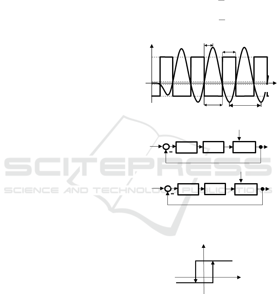
2.2 Shifting Method
A recently published method called “shifting method”
can be used for fitting a linear model (Hofreiter,
2016). This approach is based on the assumptions that
in the relay feedback experiment there is a stable
oscillation with the period T
p
(T
p
=T
1
+T
2
, T
1
≠T
2
, see
Fig. 2), the identified process is time invariant and in
the proximity of operating point has linear properties.
The block diagram for the relay feedback test is
slightly modified, see Fig. 3. Here, the additional
integrator or alternatively the transport delay D are
inserted in the closed loop (Hofreiter, 2018) and s is
the complex variable in L-transform. The shifting
method uses an asymmetrical relay with a hysteresis
(see Fig. 4) to reduce the influence of noisy
environment and for the model parameter estimation.
The basic idea of the shifting method consists in
determination of the time courses of the auxiliary
variables u
a
(t) and y
a
(t) calculated according to (1)
and (2).
2
p
a
T
u t u t u t
(1)
2
p
a
T
y t y t y t
(2)
Figure 2: The time courses u and y.
Figure 3: Block diagram of a process under relay feedback
with a) integrator b) delay D.
Figure 4: The static characteristic of an asymmetrical relay
with hysteresis.
If there are sustained oscillations in the relay
feedback test after the time t
L
then frequency points
G(jω
1
) and G(jω
2
) of a system can be estimated for
angular frequencies
u
y
y
u
T
1
T
2
T
p
u,y
ε
A
ε
B
time t
u
A
u
B
τ
m
Relay
Process
w
e
u
d
y
1/s
Relay
Process
w
e
u
d
y
e
-s·D
y
d
u
w
e
a)
b)
e
p
e
p
e
p
u
u
A
u
B
ε
A
ε
B
ICINCO 2019 - 16th International Conference on Informatics in Control, Automation and Robotics
602
12
24
,
pp
TT
(3)
where T
p
is the period of a stable oscillation using the
following formulas computed by a numerical
integration
1
1
1
,
p
p
tT
j
t
L
tT
j
t
y e d
G j t t
u e d
(4)
2
2
2
,
p
p
tT
j
a
t
L
tT
j
a
t
y e d
G j t t
u e d
(5)
where G(jω) is the process frequency transfer
function.
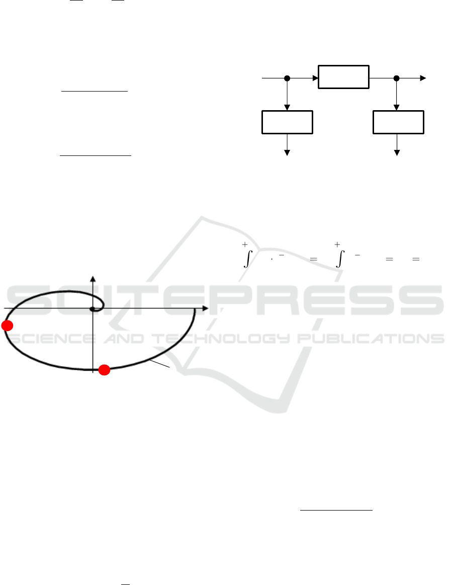
The use of a transport delay or an integrator
allows to place the points G(jω
2
) and G(jω
1
) to the 3
rd
and 4
th
quadrant (see Fig. 5). These positions are more
suitable for model fitting.
Figure 5: The Nyquist frequency characteristic of a process
and the points obtained by the shifting method.
A great advantage of the above procedure is that
the location of the points G(jω
1
) and G(jω
2
) was
determined on the basis of the relay experiment
without assuming any model structure. Therefore this
approach can be applied to models with more
parameters and different structures. The newly
acquired point G(jω
2
) determined by the shifting
method allows the estimation of two other parameters
of the model from a single relay test. It is possible due
to the use of the second order harmonic of the relay
oscillations. This follows from the relationships (1)
and (2) which describe the filter with the frequency
transfer function
2
1
p
T
j
F
G j e
(6)
Applying the filter, all odd harmonic frequencies
including the fundamental harmonic frequency
1
are
filtered out. At the same time, the even harmonic
frequencies including
2
are amplified twice (see Fig.
6).
Figure 6: The block scheme of the shifting method.
The next advantage of this approach is that the
presence of a static load disturbance with a magnitude
of d
A
does not have any influence on the calculation
G(jω
1
) and G(jω
2
) as it holds
0, 1,2
pp
ii
t T t T
jj
AA
tt
d e d d e d i
(7)
2.3 Static Gain
The static gain is often assumed to be known a priory
for estimating model parameters of proportional
systems by the relay feedback identification, e.g.
Luyben (1987) or more relay tests are necessary, e.g.
Li, Eskinat and Luyben (1991). As well, the static
gain is separately derived on the basis of the shape of
response from the relay feedback test, see Yu (1999).
Shen,Wu and Yu (1996) proposed to use an
asymmetrical relay for the static gain estimation. In
this approach the system is considered at equilibrium
at the operating point (u
0
,y
0
). If the relay feedback test
is applied on a proportional system, the static gain K
can be determined by the following formula
computed by a numerical integration
0
0
0,
p
p
tT
t
L
tT
t
y y d
K G t t
u u d
(8)
Thus, using the formulas (1), (2), (3), (4) and (5),
we obtain the three points G(0), G(jω
1
) and G(jω
2
) of
the Nyquist frequency characteristic; see Fig. 7,
which can be used for fitting the model.
G(jω
1
)
G(jω
2
)
G(jω)
Im
Re
G(jω)
G
F
(jω)
G
F
(jω)
u
y
y
a
u
a
Improved Relay Feedback Identification using Shifting Method
603

Figure 7: The Nyquist frequency characteristic of a process
and the found points G(0), G(jω
1
) and G(jω
2
).
We can use this solution in case that we know
exactly the values u
0
and y
0
. But if we do not know
them exactly, e.g. due to a static load disturbance, we
cannot use formula (8).
In case that we cannot use formula (8), the static
gain may be estimated from the found points G(jω
1
)
and G(jω
2
) obtained by the shifting method. It will be
shown in the next section.
2.4 SOTD Model
Most industrial processes can be described near the
operating point using the SOTD model with the
transfer function
21
1
u
s
Ke
Mj
a s a s
(9)
This model can be used for both oscillatory and
aperiodic systems. Additionally, it is also possible to
use this model to describe time delayed systems.
Hofreiter (2017) derived the following explicit
formulas for parameter estimation of the SOTD
model from determined values ω
1
, ω
2
, G(0), G(jω
1
)
and G(jω
2
).
0KG
(10)
22
2
2 2 2
1
21
1 1 4
3
3
2
KK
a
G j G j
(11)
2
2
2
1 2 1
2
1
1
1
1
K
aa
Gj
(12)
2
2
21
1
1
1
1
2
l
ll
u
l
l
Gj
a j a j
(13)
However, this solution can be applied only in case
we know a priory the static gain K or we can estimate
K from a single relay feedback test by formula (8). If
the static sensitivity cannot be determined by the
above mentioned procedure we can determine K and
parameters a
2
, a
1
, τ
u
using the chosen model structure
(9) and knowledge of the values ω
1
, ω
2
, G(jω
1
) and
G(jω
2
) obtained by the shifting method from a single
relay feedback test. For this purpose we can use the
following criterion
2
2
21
1
, , ,
u i i
i
Kr K a a G j M j
(14)
where M(jω) is the frequency transfer function of
model (9).
The value of the criterion Kr depends on the
values of K, a
2
, a
1
and τ
u
. For more compact notation
we introduce the vector
21
T
u
K a a
(15)
containing the unknown values of the parameter K,
a
2
, a
1
and τ
u
of the SOTD model (9). For a stable
system, the value of the vector θ that minimises the
criterion (15) can be determined by
arg min
D
Kr
(16)
where D={(K,a
2
,a
1
,τ
u
): K>0, a
2
>0, a
1
>0, τ
〈
0, 𝜏
𝑚
〉
}
and τ
m
see Fig. 2.
Denote the real and imaginary part of the complex
values G(jω
1
) and G(jω
2
)
jj
i i i
G R I
for i=1,2
(17)
then
21
1
0,
, , 0
ˆ
argmin
m
TT
u
K a a
Z Z Z p
Kr
(18)
where
2
1
1 1 1
11
2
1
1 1 1
11
2
2
2 2 2
22
2
2
2 2 2
22
cos
sin
,
cos
sin
u
u
u
u
IR
R
RI
I
Zp
IR
R
RI
I
(19)
3 SIMULATED EXAMPLE
The introduced relay identification method is
demonstrated on an aperiodic proportional process
which is taken from Berner, Hägglund and Åström
(2016). This process is described by the following
transfer function
1
1
1 0.1 1 0.01 1 0.001 1
Ps
s s s s
(20)
G(jω
1
)
G(jω
2
)
G(jω)
Im
Re
K=G(0)
ICINCO 2019 - 16th International Conference on Informatics in Control, Automation and Robotics
604
where s is the complex variable in L-transform. We
assume that the process can be described by a SOTD
model in the form (9), the relay feedback experiment
is with integrator (see Fig. 3a) and the asymmetrical
relay is with a hysteresis having the following
parameters (see Fig. 4)
2, 1, 0.1, 0.1
A B A B
uu
(21)
We will estimate the model parameters without
using the formula (8) only from the values ω
1
, ω
2
,
G(jω
1
) and G(jω
2
) obtained by a single relay feedback
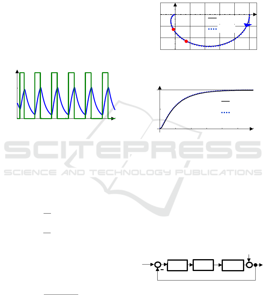
test and using the criterion (14). The time courses of
the manipulated variable u and the controlled variable
y are shown in Fig. 8.
Figure 8: The time courses of the relay output u and the
process output y obtained from the relay feedback
experiment with integrator.
Solution:
The period of stable oscillation Tp and the values ω
1
,
ω
2
, G(jω
1
) and G(jω
2
) can be determined from the
stable time courses u and y (see Fig. 8) utilizing
formulas (1), (2), (3), (4) and (5).
3.465
p
T
s (22)
1
2
1.8133
p
T
rad·s
-1
(23)
2
4
3.6267
p
T
rad·s
-1
(24)
1
0.1421 0.4533G j j
(25)
2
0.0300 0.2479G j j
. (26)
The model transfer function M
1
(s) is obtained by
minimizing the criterion (14) and the calculated
values ω
1
, ω
2
, G(jω
1
) and G(jω
2
).
0.011
1
2
1
0.1 1.1 1
s
M s e
ss
. (27)
The position of the points G(jω
1
) and G(jω
2
) together
with the Nyquist diagram of the transfer functions
P
1
(s) and M
1
(s) are shown in Fig. 9. The step
responses of the transfer functions P
1
(s) and M
1
(s) are
shown in Fig. 10. Fig. 9 and Fig. 10 show a very good
conformity between the process and its model.
Figure 9: The Nyquist diagram for the transfer functions
P
1
(s), M
1
(s) and the calculated points G(jω
1
) and G(jω
2
).
Figure 10: The step response h
P1
of the process P
1
and the
step response h
M1
of the model M
1.
Next, consider the process with the transfer
function (15) but now the relay feedback
identification is realized under a constant load
disturbance d where
0.5d
(28)
The process is controlled by the asymmetrical relay
with integrator, see Fig. 11. The time courses of the
manipulated variable u and the controlled variable y
are shown in Fig. 12. The goal is to approximate the
process transfer function by the SOTD model.
Figure 11: The process under the load disturbance d
controlled by the asymmetrical relay with integrator.
0
5
10
15
20
-1
0
1
2
u
y
time [s]
u,y
-0.2
0
0.2
0.4
0.6
0.8
1
-0.6
-0.4
-0.2
0
0.2
P
1
(jω)
Re
Im
G(jω
2
)
G(jω
1
)
M
1
(jω)
0
1
2
3
4
5
6
0
0.5
1
h
P1
h
M1
h
P1
,h
M1
time [s]
Relay
Process
w
e
u
d
1/s
y
d
u
w
e
e
p
Improved Relay Feedback Identification using Shifting Method
605
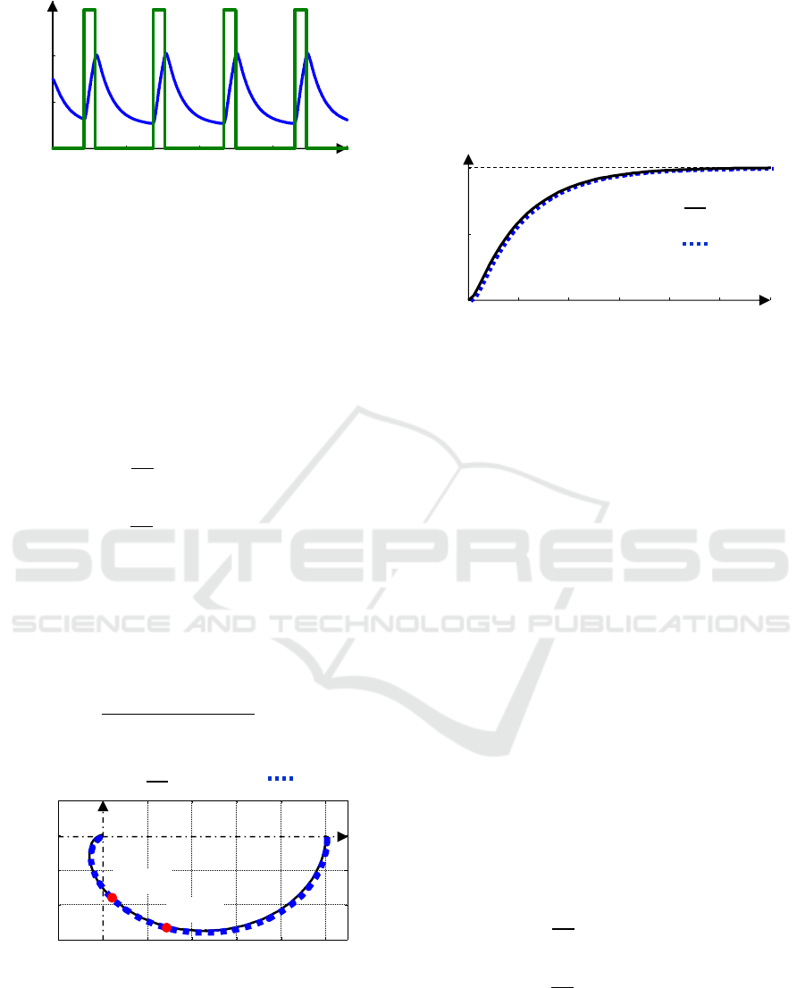
Figure 12: The time courses of the relay output u and the
process output y obtained from the relay feedback
experiment with integrator under the static load
disturbance.
Solution:
The period of stable oscillation Tp and the values ω
1
,
ω
2
, G(jω
1
) and G(jω
2
) can be determined from the
stable time courses u and y (see Fig. 12) utilizing
formulas (1), (2), (3), (4) and (5).
4.805
p
T
s (29)
1
2
1.3076
p
T
rad·s
-1
(30)
2
4
2.6153
p
T
rad·s
-1
(31)
1
0.2928 0.5262G j j
(32)
2
0.0276 0.3440G j j
. (33)
The model transfer function M
5
(s) is obtained by
minimizing the criterion (14) and the calculated
values ω
1
, ω
2
, G(jω
1
) and G(jω
2
).
0.00964
2
2
1
0.1017 1.102 1
s
M s e
ss
. (34)
Figure 13: The Nyquist diagram for the transfer functions
P
1
(s), M
2
(s) and the calculated points G(jω
1
) and G(jω
2
).
The position of the points G(jω
1
) and G(jω
2
)
together with the Nyquist diagram of the transfer
functions P
1
(s) and M
2
(s) are shown in Fig. 13. The
step responses of the transfer functions P
1
(s) and
M
2
(s) are shown in Fig. 14. Although the static load
disturbance d affects the period of sustained
oscillations (see Fig. 8 and Fig. 12 or relations (22)
and (29)), its effect is eliminated when calculating
G(jω
1
) and G(jω
2
) with respect to relation (7). This is
a very important feature for practice.
Figure 14: The step response h
P1
of the process P
1
and the
step response h
M2
of the model M
2
.
4 LABORATORY EXPERIMENT
The introduced method was also verified on a
laboratory apparatus “Air Aggregate”, see Fig. 15.
The apparatus consists of a ventilator and a flow rate
meter located in a tunnel. The desired value of air
flow is maintained by the asymmetrical relay with
integrator. The manipulated variable (power to the
ventilator) u and the controlled variable (air flow) y
are provided via unified electrical signals (0-10 V).
The time courses of the biased relay output u and the
output y are shown in Fig. 16. The goal is to
approximate the process transfer function by the
SOTD model.
Solution:
The period of stable oscillation Tp and the values ω
1
,
ω
2
, G(jω
1
) and G(jω
2
) can be determined from the
stable time courses u and y (see Fig. 16) utilizing
formulas (1), (2), (3), (4) and (5).
46.5
p
T
s (35)
1
2
0.1351
p
T
rad·s
-1
(36)
2
4
0.2702
p
T
rad·s
-1
(37)
1
0.2416 1.2674G j j
(38)
2
0.4809 0.6787G j j
. (39)
0
5
10
15
20
-1
0
1
2
u,y
u
y
time [s]
-0.2
0
0.2
0.4
0.6
0.8
1
-0.4
-0.2
0
0.2
G(jω
2
)
G(jω
1
)
P
1
(jω)
M
2
(jω)
Re
Im
0
1
2
3
4
5
6
0
0.5
1
h
P1
h
M2
time [s]
h
P1
, h
M2
ICINCO 2019 - 16th International Conference on Informatics in Control, Automation and Robotics
606
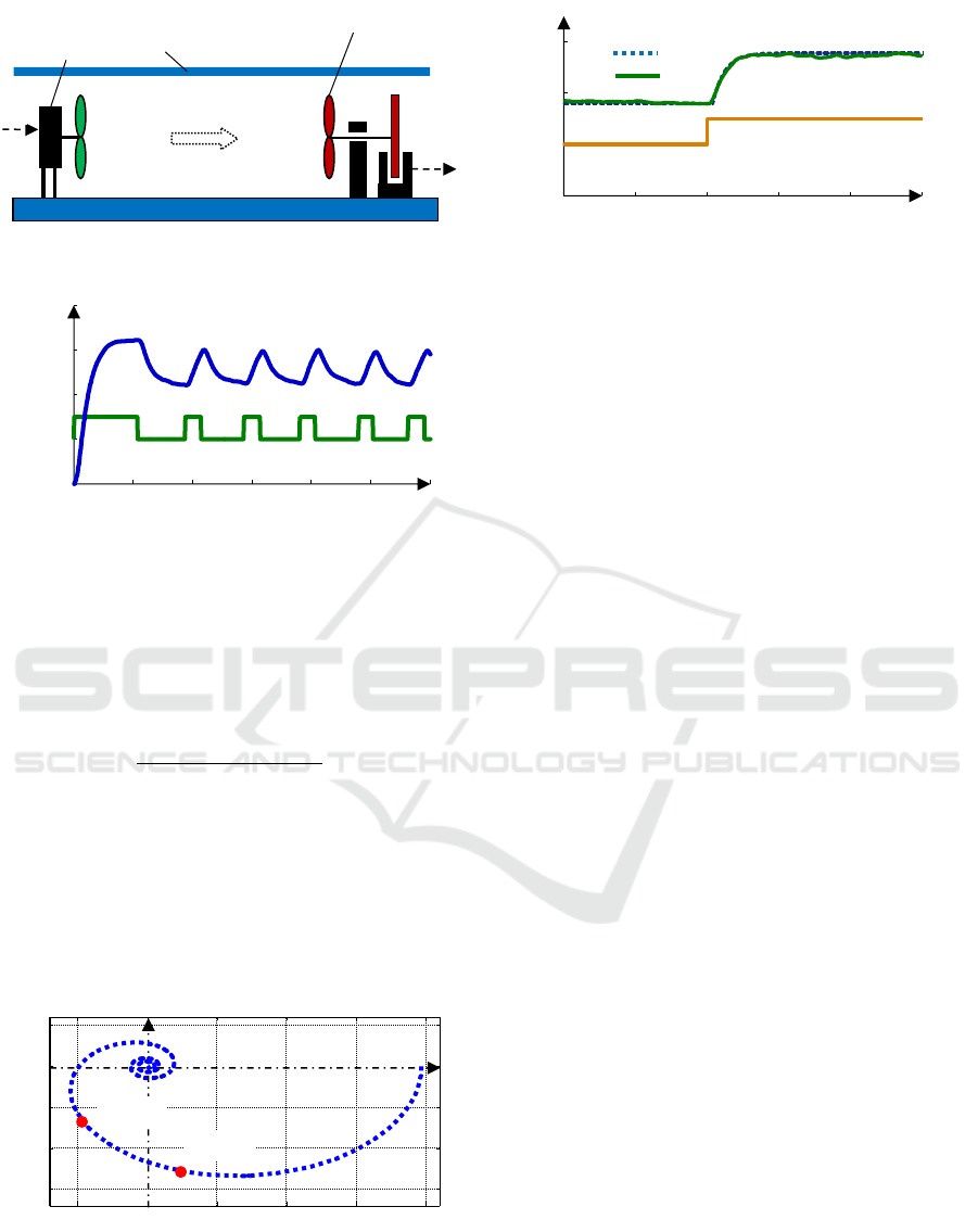
Figure 15: The laboratory apparatus “Air Aggregate”.
Figure 16: The time courses of the relay output u and the
process output y obtained from the relay feedback
experiment with integrator.
The model transfer function M
T
(s) is obtained by
minimizing the criterion (14) and the calculated
values ω
1
, ω
2
, G(jω
1
) and G(jω
2
).
3.89
2
1.969
0.0044 8.315 1
s
T
M s e
ss
. (40)
The position of the points G(jω
1
) and G(jω
2
) together
with the Nyquist diagram of the transfer function
M
T
(s) are shown in Fig. 17. The step responses of the
identified process y and the model output y
M
on the
manipulated variable u are shown in Fig. 18. Fig. 17
and Fig. 18 show a very good conformity between the
process and its model.
Figure 17: The Nyquist diagram for the transfer functions
M
T
(s) and the calculated points G(jω
1
) and G(jω
2
).
Figure 18: The time courses of the manipulated variable u,
the model output y
M
and the process output y.
5 CONCLUSIONS
The introduced relay identification method has the
following important properties:
The shifting method can be applied if in the relay
feedback experiment there is a stable oscillation
with the period T
p
(T
p
=T
1
+T
2
, T
1
≠T
2
, see Fig. 1),
the identified process is time invariant and in the
proximity of operating point has linear properties.
This approach enables to obtain two frequency
response points G(jω
1
) and G(jω
2
) using a single
relay test.
The obtained frequency points G(jω
1
) and G(jω
2
)
are determined without any assumption about a
model.
The constant load disturbance has no effect on the
positions of the frequency points G(jω
1
) and
G(jω
2
).
The identification method is primarily proposed for
automatic tuning of controllers.
The method enables to estimate all the parameters
of the SOTD model from a single relay feedback
test.
By using the SOTD model, it is possible to estimate
the static gain even in the presence of a constant
load disturbance.
The shifting method can be used both for
overdamped/underdamped systems and also for
time delayed systems.
Noisy environment is reduced by using the
asymmetrical relay with a hysteresis.
The calculation of relations (4) and (5) can be
refined by integration over multiple periods T
p
.
y
u
Covering tunnel
Ventilator
Propeller flow meter
0
50
100
150
200
250
300
0
2
4
6
8
u
y
u,y
time [s]
-0.5
0
0.5
1
1.5
2
-1.5
-1
-0.5
0
0.5
G(jω
2
)
G(jω
1
)
Re
Im
0
50
100
150
200
250
0
2
4
6
y
M
y
u
u,y
M
,y
P
[V]
time [s]
Improved Relay Feedback Identification using Shifting Method
607

ACKNOWLEDGMENT
The presented work was supported by the
Institutional Resources of CTU in Prague for research
(RVO12000).
REFERENCES
Åström, K. J. and Hägglund, T. (1984). Automatic tuning
of simple regulators with specifications on phase and
amplitude margins. Automatica, 20 (5), pp. 645-651.
Berner, J., Hägglund, T. and Åström, K. J. (2016).
Improved relay autotuning using normalized time
delay. American Control Conference (ACC), IEEE, pp.
1869-1875.
Chidambaram M. and Sathe V. (2014). Relay Autotuning
for Identification and Control. Cambridge University
Press, Cambridge.
Hofreiter, M. (2016). Shifting method for relay feedback
identification. IFAC-PapersOnLine, 49 (12), pp. 1933-
1938.
Hofreiter, M. (2017). Biased-relay feedback identification
for time delay systems, IFAC-PapersOnLine, 50 (1),
pp. 1462-14625.
Hofreiter, M. (2018). Alternative identification method
using biased relay feedback, IFAC-PapersOnLine, 51
(11), pp. 891-896.
Kalpana, D. and Thyagarajan, T. (2018). Parameter
estimation using relay feedback. Reviews in Chemical
Engineering, De Gruyter, Berlin.
Li W., Eskinat E. and Luyben W. L. (1991). An improved
auto-tune identification method, Ind. Eng. Chem. Res.
30 (7), pp. 1530-1541.
Liu T. and Gao F. (2012). Industrial process identification
and control Design: Step-test and relay-experiment-
based Method. Advances in Industrial Control.
Springer-Verlag, London.
Liu T., Wang Q. G. and Huang H. P. (2013). A tutorial
review on process identification from step or relay
feedback test. Journal of Process Control, 23 (10), pp.
1597-1623.
Luyben, W. L. (1987). Derivation of transfer functions for
highly nonlinear distillation columns. Ind. Eng. Chem.
Res. 26 (12), pp. 2490-2495.
Ruderman, M. (2019). Relay feedback systems-established
approaches and new perspectives for application, IEEJ
J. of Industry Applications. 8 (2), pp.271-278.
Shen, S. H., Wu, J. S. and Yu C. C. (1996). Use of biased-
relay feedback for system identification. AIChE. J. 42
(4), pp. 1174-1180.
Yu C. C. (1999). Autotuning of PID Controllers, ch. 2 and
3. Springer-Verlag, London.
Ziegler J. G. and Nichols N. B. (1943). Optimum settings
for automatic controllers. Trans. ASME, vol. 65, pp.
433-444.
ICINCO 2019 - 16th International Conference on Informatics in Control, Automation and Robotics
608
