Recommendations from Cold Starts in Big Data

David Ralph

1 a

, Yunjia Li

2 b

, Gary Wills

1 c

and Nicolas G. Green

1 d

Electronics and Computer Sciences (ECS), University of Southampton, University Rd, Southampton, SO17 1BJ, U.K

Launch International LTD, 3000a Parkway, Whiteley, Fareham, PO15 7FX, U.K

Keywords: Recommender Systems, Information Retrieval, Data Mining, Sparse Data, Partially Labelled Data.

Abstract: In this paper, we introduce Transitive Semantic Relationships (TSR), a new technique for ranking

recommendations from cold-starts in datasets with very sparse, partial labelling, by making use of semantic

embeddings of auxiliary information, in this case, textual item descriptions. We also introduce a new dataset

on the Isle of Wight Supply Chain (IWSC), which we use to demonstrate the new technique. We achieve a

cold start hit rate @10 of 77% on a collection of 630 items with only 376 supply-chain supplier labels, and

67% with only 142 supply-chain consumer labels, demonstrating a high level of performance even with

extremely few labels in challenging cold-start scenarios. The TSR technique is generalisable to any dataset

where items with similar description text share similar relationships and has applications in speculatively

expanding the number of relationships in partially labelled datasets and highlighting potential items of interest

for human review. The technique is also appropriate for use as a recommendation algorithm, either standalone

or supporting traditional recommender systems in difficult cold-start situations.

1 INTRODUCTION

New Big Data recommendation systems face a high

barrier to entry due to the large labelled data

requirement of most existing recommendation

techniques such as collaborative filtering and bespoke

deep learning models such as Suglia et al., (2017).

Obtaining this labelled data, such as user interactions

or human judgements, is particularly problematic in

highly specialised or commercially competitive

domains where this labelling may not yet exist or not

be freely available, often requiring an expensive

expert or crowd-sourced labelling. As such,

techniques that function well with few labels are

highly desirable.

The cost of labelling is highly dependent on the

complexity of the task, specifically the time needed

per human annotation and the expertise required.

Snow et al., (2008) find that for tasks such as textual

entailment and word sense disambiguation

approximately four non-expert labels have similar

quality to one expert label. Grady and Lease (2010)

investigate crowdsourcing binary relevance labelling

https://orcid.org/0000-0003-3385-9295

https://orcid.org/0000-0002-5728-9795

https://orcid.org/0000-0001-5771-4088

https://orcid.org/0000-0001-9230-4455

tasks and find that tasks where annotators must use

item descriptions achieve poorer accuracy and require

greater time per judgement than tasks using titles.

In some cases, datasets may be too large for

comprehensive manual labelling and may only be

viable to label by observing user behaviour, which

requires a system able to function with very few

labels without exclusively preferencing the already

labelled subset of the data. Such systems can be used

to bootstrap a recommendation platform where user

interactions can then be observed to enhance the

model or train an alternative model which performs

well with many labels. This is also related to the cold-

start problem where newly added items have no past

interaction data.

Content based and hybrid recommender systems

reduce the requirement for user-item interaction

labels by making use of item content, such as

descriptions. Many such systems rely on either

knowledge bases and ontologies (Zhang et al., 2016),

which do not avert the requirement of experts for new

or commercially guarded domains, or tags and

Ralph, D., Li, Y., Wills, G. and Green, N.

Recommendations from Cold Starts in Big Data.

DOI: 10.5220/0007798801850194

In Proceedings of the 4th International Conference on Internet of Things, Big Data and Security (IoTBDS 2019), pages 185-194

ISBN: 978-989-758-369-8

185

categorisation (Xu et al., 2016), which requires either

many labels or distinct groupings in the data.

2 ISLE OF WIGHT SUPPLY

CHAIN DATASET

We examine the case of supply chain on the Isle of

Wight. We introduce a new dataset for this task,

which we name the Isle of Wight Supply Chain

(IWSC) dataset. The data consists of varying length

text descriptions of 630 companies on the Isle of

Wight taken via web scraping from the websites of

IWChamber (2018), IWTechnology (2018), and

Marine Southeast (2018).

HTML tags and formatting have been

removed, but the descriptions are otherwise unaltered

and are provided untokenized, without substitutions,

and complete with punctuation. Some descriptions

contain product codes, proper nouns, and other non-

dictionary words.

Most of the descriptions are a few sentences

describing the market role of the company, or a

general description of the company’s activities or

products. Several but not all the descriptions also

contain a list of keywords, but this is included as part

of the descriptive text and not as an isolated feature.

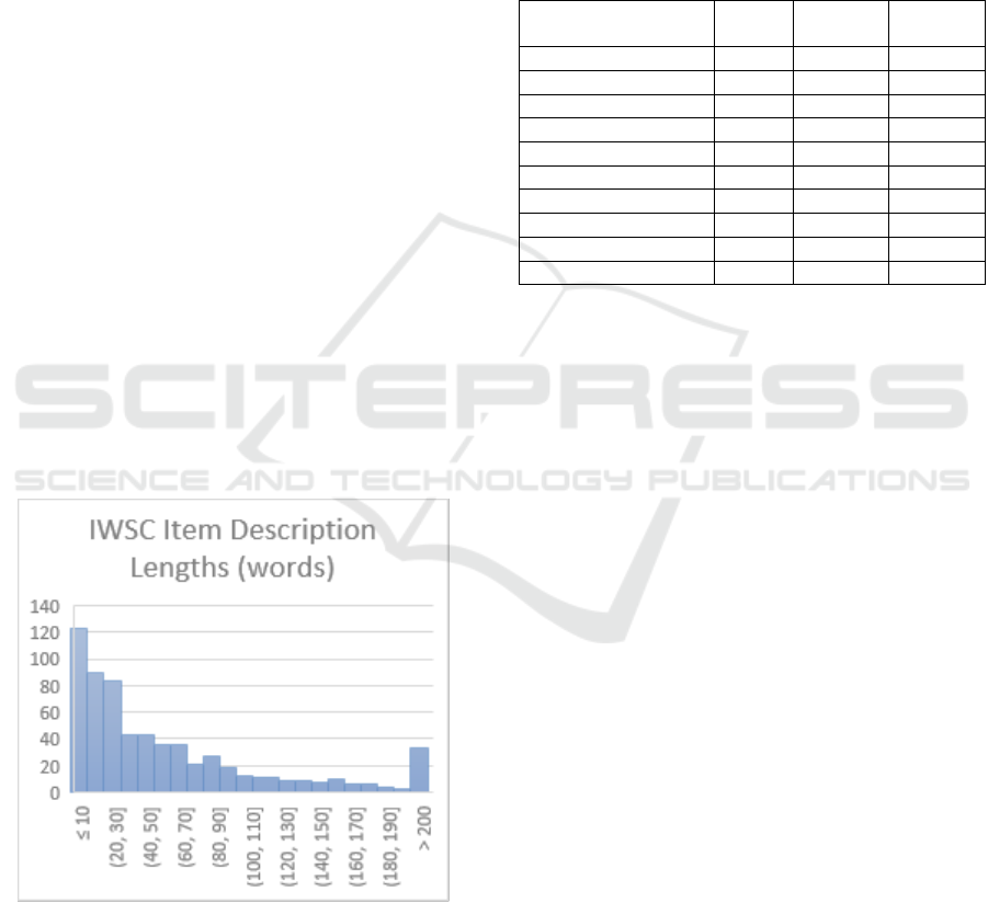
The mean description length is 61 words, or 412

characters (including whitespace). The distribution of

description lengths is shown in Figure 1.

Figure 1: Histogram of item description lengths in the

IWSC dataset.

The IWSC dataset is provided with two discrete

sets of labels intended to evaluate algorithmic

performance in different scenarios. In both cases, the

labels are binary, directed, human judgements of

market relatedness based on the company

descriptions. The number and distribution of labels is

shown in Table 1. These labels are speculative

potential relationships, not necessarily real existing

relationships. We choose to provide binary labels as

real-world supply chain relationships are typically

multi-class binary relationships. i.e. any two

companies either are or are not in each possible type

of supply chain relationship.

Table 1: Labels in the IWSC dataset.

Label Name

Total

Labels

Labelled

Items

Unique

Targets

SL_suppliers

142

SL_not_suppliers

563

120

SL_consumers

376

117

SL_not_consumers

712

157

SL_competitors

SL_not_competitors

396

ES_suppliers

ES_consumers

207

171

ES_competitors

ES_unrelated

431

299

The first label set we denote IWSC-SL. It is

comprised of the labels ‘SL_consumers’,

‘SL_not_consumers’, ‘SL_suppliers’,

‘SL_not_suppliers’, ‘SL_competitors, and

‘SL_not_competitors. These labels are concentrated

on a small number of labelled items, relating them to

a random distribution of other items (both labelled

and unlabelled). These labels are intended for

evaluation in the case that we only have records for a

small subset of items and must extrapolate from this

to perform inferences on many unseen items. We

refer to this scenario as “Subset Labelling” (SL).

The second label set we denote IWSC-ES. It is

comprised of the labels ‘ES_suppliers’,

‘ES_consumers’, ‘ES_competitors’, and

‘ES_unrelated’. The labels are randomly distributed

across all labelled items with no intentional patterns

(random pairs were selected for labelling). These

labels are intended for evaluation in the case that

known items have very few labels and many are

entirely unlabelled, in contrast to common

recommender system datasets such as Movie

Reviews (MR) (Pang and Lee, 2004), Customer

Reviews (CR) (Hu and Liu, 2004), and MovieLens

(Harper and Konstan, 2015), where most items have

many recorded interactions. While in those examples

the labels are sparse as most possible item pairs are

unlabelled, in our scenario, which we refer to as

“extremely sparse” (ES) labelling, there is the

additional condition that most items in the dataset do

not occur in any of these pairs.

IoTBDS 2019 - 4th International Conference on Internet of Things, Big Data and Security

186

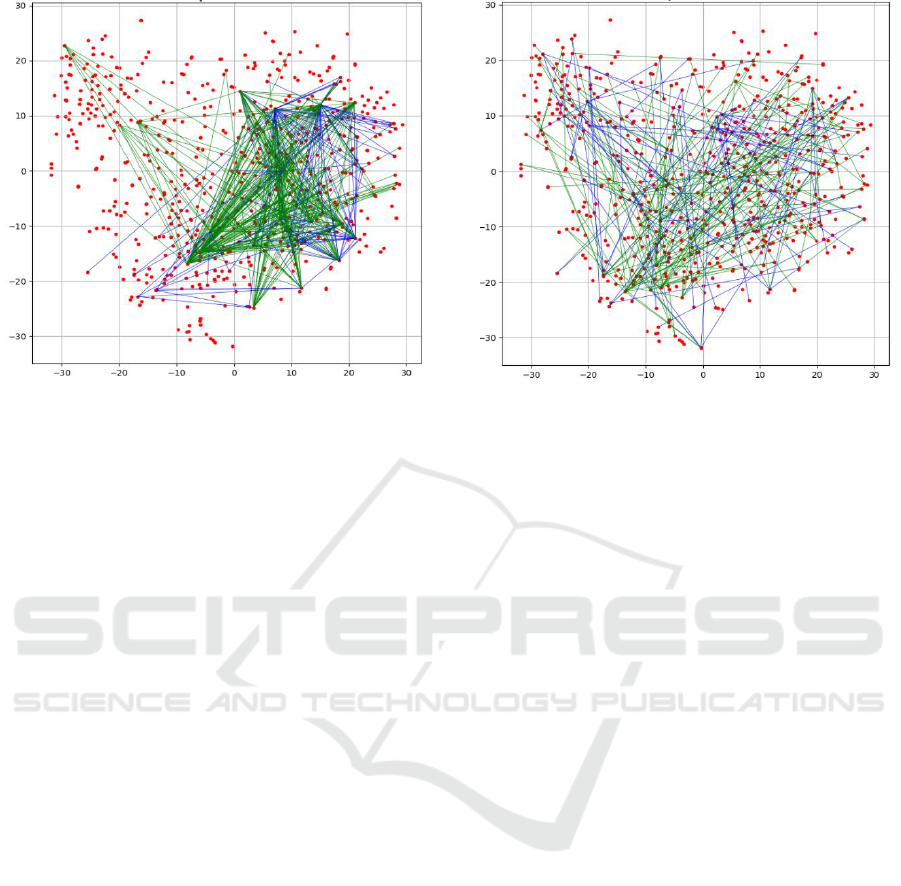
Figure 2: A 2D t-SNE plot of ISWC item description

embeddings showing labels for the SL tasks.

Figures 2 and 3 illustrate the label distributions

using 2d t-SNE (Maaten and Hinton, 2008) plots of

IWSC item description embeddings generated using

Universal Sentence Encoder (USE) (Cer et al., 2018),

annotated with the labels from IWSC-SL and IWSC-

ES respectively.

For the problem of effective recommendations

from few labels, we set the four following tasks:

1. Prediction of “SL_consumers” labels using

IWSC-SL labels and item descriptions

2. Prediction of “SL_suppliers” labels using IWSC-

SL labels and item descriptions

3. Prediction of “ES_consumers” labels using

IWSC-ES labels and item descriptions

4. Prediction of “ES_suppliers” labels using IWSC-

ES labels and item descriptions

These tasks could also be expressed as two multi-

class classification problems (one each for IWSC-SL

and IWSC-ES), but in this paper we look at the four

single-class recommendation tasks set out above.

The full IWSC dataset is available for download

from https://github.com/DavidRalph/TSR-Public/

tree/master/datasets

3 TRANSITIVE SEMANTIC

RELATIONSHIPS

We introduce a novel approach to approach the

problems of extremely sparse labelling and subset

labelling previously described, that we call

“Transitive Semantic Relationships” (TSR). TSR

uses auxiliary item information for unsupervised

Figure 3: A 2D t-SNE plot of ISWC item description

embeddings showing labels for the ES tasks.

comparison of items to expand the coverage of the

few available labels. This is conceptually similar to

other embedding based hybrid recommenders such as

Vuurens et al. (2016) and He et al. (2017), but we

implement a novel approach which combines item

content embeddings with inferential logic instead of

learned or averaged user embeddings, making it

suitable for datasets with fewer labels and producing

provenance that is both intuitively understandable

and easy to visualise.

3.1 Theory

Transitive Semantic Relationships are based on an

apparent transitivity property of many types of data

items, where it is the case that items which are

described similarly are likely to have similar

relationships to other data items. Take for example,

the supply chain: if company A, a steel mill and

company B, a construction firm are known to have the

relationship A supplies (sells to) B, it is likely that

some other companies C, another steel mill, and D,

another construction firm, would have a similar

relationship. Given auxiliary information about each

company, such as a text description of their product

or market role, and the example relationship A->B,

we can infer the potential relationships C->D, A->D,

and C->B. We illustrate this example in Figure 4.

It follows that the greater the similarity between

an item of interest and an item in a known

relationship, the greater confidence we can have that

the relationship is applicable. Given some fixed

length vector representation of the auxiliary

information about each item, we can use cosine

Recommendations from Cold Starts in Big Data

187

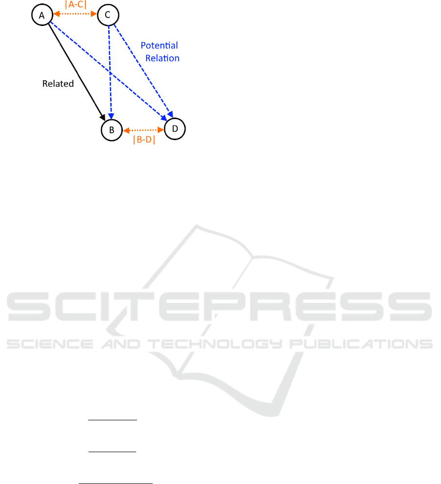
Figure 4: Illustration of Transitive Semantic Relationships.

similarity to measure similarity between the items.

The vector representation should ideally capture

semantic features of the auxiliary information that

indicate whether the items they describe are similar in

function in terms of the known relationship. If the

vector representations fulfil this criterion, then the

cosine similarity between two items is their semantic

similarity. It then follows that we can determine the

confidence that two items share a relationship by

measuring the cosine similarity of the semantic vector

for each item with another pair of items that share the

same relationship. Cosine similarity values range

from 0 (no similarity) to 1 (completely similar), so to

keep confidence scores in the range 0 to 1, we take

the sum of the similarity values over 2.

Continuing from the prior example illustrated in

Figure 4, if the semantic similarity of A and C is |A-

C|, and the similarity of B and D is |B-D|, we can

calculate the confidence for each inferred relationship

to be as shown in equations 1, 2, and 3.

   

 



  







(1)

   



  



 





(2)

   



 







  





(3)

To further illustrate this, if C is very similar to A,

for example |A-C|=0.8, but D was only slightly

similar to B, |B-D|=0.2, then we can calculate A-

>D=0.6, C->B=0.9, C->D=0.5, indicating that there

is a good chance that C could share a similar

relationship with B as A does, but other new relations

are unlikely. In another example, if C remains very

similar to A, |A-C|=0.8, and we make D highly similar

to B, |B-D|=0.7, then we calculate A->D=0.85, C-

>B=0.9, C->D=0.75, showing that while all

relationships are likely, higher confidence scores are

awarded when there is less uncertainty (due to

dissimilarity with the known items).

Taking the inverse of this TSR confidence can be

described as the combined-cosine-distance, or more

generally the combined-semantic-distance. When

explaining algorithms for recommendation using

TSR confidence, we generally use this combined

distance metric as we consider it easier to interpret

when results are visualised and when distance values

are weighted.

3.2 Application

The previous scenarios suppose that we have already

pre-determined the items of interest for comparison.

However, we can extend this principle to selection of

items for comparison, given an input item to use as a

query. Note that this is not a query in the sense of

traditional search engines but is auxiliary information

for an item for which we want to find relations (e.g.

an item description).

First, we must make the distinction between cases

where relationships map from one space to some

other non-overlapping space, for example separate

document collections, and the alternative case where

items on either side of the relationship co-exist in the

same space. A practical example of the former might

be a collection of resumes and a collection of job

adverts, while an example of the later might be

descriptions of companies looking for supply chain

opportunities, as in the IWSC dataset on which we

evaluate TSR later in this paper. The TSR scoring

does not differentiate between these two dataset

types, but in the former case, with separate item

collections, it is only necessary to make similarity

comparisons between items in the same collection

and irrespective of the total number of collections, we

need only examine the collections featuring items on

either end of at least one example of the relationship

type of interest; this may be a useful filtering criteria

in datasets featuring many types of relationships

across many non-overlapping collections.

Having identified the collections that are of

interest, we can optionally apply additional filtering

of items before similarity comparison, such as by

using item meta-data or additional auxiliary

information, for example, only considering recent

information, or limiting by language or region. This

filtering could be done to the list of known

relationships, if, for example historical trends are not

of interest, or could be applied to potential targets, for

example, ignoring adverts in a different language to

the query item.

IoTBDS 2019 - 4th International Conference on Internet of Things, Big Data and Security

188

The next stage is to calculate similarity between

the query item and other items in the same collection

which are members of relationships of the type we are

looking to infer, items not in such relationships are

not of interest. We then calculate the similarity

between the query and each of these, we refer to these

items as “similar nodes” and call the similarity for

each S1.

We then look at all items pointed to by the known

relationships of each similar node, we refer to these

collectively as “related nodes”. If the number of

similar nodes is large we can choose to only follow

relationships for a maximum number of similar

nodes, preferring ones most similar to the query, in

the results section we denote this parameter as L1. We

then calculate the similarity between each related

node and every other node in that space, which we

call the “target nodes” and the similarity S2. An item

can be both a related node and a target node, but an

item cannot be both the query and a target node. If the

number of target nodes is large, we can limit the

number of comparisons in the next stage by

considering only a maximum number of targets for

each related node, preferring the most similar, we

denote this parameter as L2.

We discuss alternative scoring approaches in

section 5.3, but a simple scoring metric equivalent to

the pre-selected items examples in the previous

section is to determine the score for each target node

by finding the largest value for (S1+S2)/2 that creates

a path to it from the query item, where S1 is the

similarity between the query and an item in the

query’s space (the similar node), which shares a

relationship with an item in the target’s space (the

related node) which is of similarity S2 to the target

node. This scoring system ranks items by the

minimum combined-semantic-distance from a known

relationship of the desired type.

In Figure 5 we show a visualised example of

several TSR routes for a query. Due to the number of

relationships considered for a query a 2d plot is not

an ideal visualisation. While not shown in this

publication, the evaluation software can also produce

interactive 3d plots which allow inspection of

individual routes and the relevant nodes and labels,

allowing some insight into the behaviour of the

scoring algorithm.

Figure 5: A 2D t-SNE plot of IWSC item descriptions

showing labelled and inferred relationships for a query.

Each route is comprised of three lines: query node→similar

node, similar node→related node, related node→target

node.

4 EVALUATION TECHNIQUES

Various evaluation metrics are used in recommender

system and information retrieval literature. As the

IWSC dataset uses binary labels, and the total number

of labels is small, we look at evaluation techniques

which best reflect this.

Normalised Discounted Cumulative Gain

(NDCG) (Järvelin and Kekäläinen, 2002) is a

common evaluation metric in information retrieval

literature. This is a graded relevance metric which

rewards good results occurring sooner in the results

list, however it does not penalise highly ranked

negative items. As binary labels have no ideal order

for positive items, we do not consider this a suitable

metric.

Quantitative error metrics such as Root Mean

Squared (RMS) error or Median Absolute Error are

also common. Error metrics naturally favour scoring

systems optimised to minimise loss such as learning-

to-rank algorithms and require scores to fit the same

range as the label values. For the IWSC dataset, as the

labels are binary, the range is 0 to 1. However, scores

output from TSR have no guarantee of symmetric

distribution over the possible output range and are

typically concentrated towards high-middle values

due to averaging similarity scores making extreme

values uncommon. Figure 6 shows the typical score

distribution for the standard TSR algorithm TSR-a.

In section 5.3 we describe some alternative

scoring algorithms with unbounded upper values. A

scaling function can be applied after scores are

calculated to fit them to a specific range, but this still

Recommendations from Cold Starts in Big Data

189

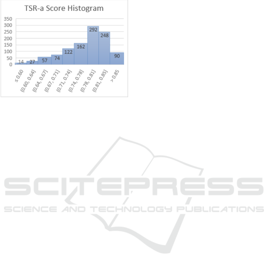
Figure 6: Histogram of item scores produced by TSR-a.

does not guarantee the desired distribution and could

be sensitive to outliers, such as unusually high scoring

items, distorting error values.

For a binary labelled dataset, it is intuitive to set

some threshold on the rankings and produce a

confusion matrix, and take precision (P), recall (R),

and f1 scores. As scores are not evenly distributed,

there is no obvious score value to use as a threshold,

so instead we look at some number of the top ranked

items.

Due to the sparsity of labels in the dataset, the

number and ratio of known positives and known

negatives varies significantly between items and in

many cases the number of known positives is smaller

than typical values of K used for Precision at K. For

this reason, we instead use R-Precision, setting the

threshold at R, the number of true positives, and take

the R most highly rated items to be predicted positive

and all remaining to be predicted negative; at this

threshold P, R, and f1 are equal. In the results section,

we denote scores taken at this threshold as @R. A

drawback of this approach is that we can only

evaluate using known positives and known negatives,

which is a minority of possible pairs in a sparse

dataset. The difficulty of this evaluation task also

varies with the ratio of known positives and negatives

which is undesirable when evaluating datasets such as

IWSC where the ratio varies greatly between items.

Finally, we look at techniques from the literature

on implicit feedback. Techniques for implicit

feedback have the desirable property of allowing us

to expand the number of unique evaluation cases by

enabling us to use unlabelled pairs of items (which for

a sparse dataset is most possible item pairs) as

implicit negative feedback. We use the common

evaluation framework used by He et al. (2017) and

Koren (2008), where we perform leave-one-out cross

validation by, for each item, taking one known

positive and 100 randomly selected other items

(excluding known positives), and judging the ranking

algorithm by ability to rank the known positive

highly. The typical threshold used is that the known

positive must be in the top 10 results, this Hit Ratio

(HR) metric is denoted as HR@10. HR@5 refers to

the known positive being in the top 5, and HR@1 as

it being the highest rated item. We also show the

mean and median values for the ranks of the known

positives across all test cases.

It is of note that due to the random selection of

negative items results may vary between runs. To

ensure the results are representative we test each

known positive against multiple random pools of

implicit negatives. This significantly increases the

compute time required for evaluation but minimises

variation in scores between runs.

Having a fixed number of items in each evaluation

and repeating with different random sets of items

makes this metric well suited to datasets with uneven

label distribution such as IWSC. We also consider the

values to be quite intuitive as the random-algorithm

performance for any HR@n is approximately n%,

with ideal performance always being 100%. Mean

and median positive label rank is in the range 0 to 100.

5 RESULTS

We first use a neural language model to generate

fixed length embeddings for all descriptions. In this

study we use Universal Sentence Encoder (USE).

This model was chosen as it shows good performance

on a range of existing downstream tasks (Cer et al.,

2018). It is also of particular interest that this model

was fine-tuned on the SNLI dataset (Bowman et al.,

2015), a set of sentence pairs labelled as

contradiction, entailment, or unrelated; we speculate

that this may require the model to learn similar

linguistic features as are likely needed for the supply

chain inference task as the ability to discern whether

pairs of descriptions are entailed or contradictory is

essential to human judgements for this task, in

particular, in determining if companies serve similar

supply chain roles. As the focus of this paper is in

introducing TSR, we leave detailed investigation of

the effects of upstream embedding models to future

work.

IoTBDS 2019 - 4th International Conference on Internet of Things, Big Data and Security

190

Table 2: Explicit feedback evaluation of TSR-a on the IWSC-SL tasks.

Positive Label

Name

Labelled

Items

Positive

Labels

Negative

Labels

RMS

Error

Median Absolute

Error

SL_consumers

375

712

0.520

0.204

0.688

SL_suppliers

142

525

0.477

0.234

0.682

Table 3: Implicit feedback evaluation of TSR-a on the IWSC-SL tasks.

Positive Label

Name

Labelled

Items

Positive

Labels

@10

Median

Positive Rank

Mean Positive

Rank

SL_consumers

376

0.752

0.510

0.146

7.8

SL_suppliers

142

0.663

0.543

0.150

14.0

Table 4: Explicit feedback evaluation of TSR-a on the IWSC-ES tasks.

Positive Label

Name

Labelled

Items

Positive

Labels

Negative

Labels

RMS

Error

Median Absolute

Error

ES_consumers

115

198

0.549

0.167

0.560

ES_suppliers

259

0.350

0.177

0.572

Table 5: Implicit feedback evaluation of TSR-a on the IWSC-ES tasks.

Positive Label

Name

Labelled

Items

Positive

Labels

@10

Median

Positive Rank

Mean Positive

Rank

ES_consumers

207

0.221

0.119

0.018

43.0

ES_suppliers

0.197

0.129

0.055

47.7

5.1 Results for Subset Labelled Tasks

Table 2 and Table 3 show our results on the two

IWSC-SL tasks introduced in section 2. In these

experiments we used the least-combined-cosine-

distance soring metric described in section 3.2 and

evaluate using metrics discussed in section 4. All

experiments are cold-start scenarios where the input

(query) item is treated as unseen, only the USE

embedding of its description is known.

We set the parameters L1=5 and L2=10, for this

scoring metric the value of these parameters has little

impact on performance as only the best routes

contribute to scoring, but it is observable that this

inflates the mean positive rank as items lacking good

routes are more excluded from the results, which we

treat as it being the worst possible rank.

For the implicit feedback evaluations (HR and

Positive Rank) we use one known positive, and a

random pool of 100 not-known-positive items. We

repeat this process 10 times for each label, using

different random pools, and calculate the scores

across all tests. Therefore, the number of test runs is

always 10 times the number of positive labels. The

number of labelled items and positive labels used in

the implicit feedback tests is higher as we can

additionally test items that lack any known negatives.

Our results show good performance on the IWSC-

SL tasks, considering how few labels are available,

achieving a hit-rate@10 of over 75%. It is notable that

we see less than 9% worse performance on the

SL_suppliers test despite having less than half the

number of labels, showing that the algorithm can

achieve good performance on labelled-subset tasks

even when extremely few labels are available (142

labels in a dataset of 630 items). For both IWSC-SL

tasks the frequency of the top ranked item being the

known positive (when competing with 100 randomly

selected others) HR@1 appears similar and is 14-15

times better than random.

5.2 Results for Extra Sparse Labelling

Tasks

Table 4 and Table 5 show our results on the two

IWSC-ES tasks introduced in section 2. The

algorithm and parameters are the same as in the

IWSC-SL tasks tests. The IWSC-ES tasks each have

around half the number of positive labels as the

IWSC-SL tasks, so a lower score should be expected.

In the IWSC-ES tasks we show significantly

worse hit-rate, but smaller median absolute error and

RMS error. We speculate that the lack of dense

regions in the labels, due to the extreme sparsity and

random distribution, makes identifying a particular

Recommendations from Cold Starts in Big Data

191

Table 6: Evaluation of alternative TSR algorithms on the IWSC SL_consumers task.

Scoring

Algorithm

@10

Median

Positive

Rank

Mean

Positive

Rank

RMS

Error

Median

Absolute

Error

TSR-a

0.754

0.509

0.145

7.7

0.520

0.204

0.688

TSR-a*

0.754

0.509

0.145

7.7

0.520

0.195

0.481

TSR-b

0.548

0.364

0.115

11.5

0.541

0.12

0.319

TSR-c

0.573

0.385

0.133

10.9

0.544

0.12

0.309

TSR-d

0.565

0.373

0.124

11.1

0.544

0.122

0.322

TSR-e

0.771

0.532

0.163

7.6

0.530

0.204

0.584

TSR-f

0.582

0.408

0.158

10.5

0.549

0.146

0.456

TSR-g

0.742

0.536

0.185

7.8

0.533

0.192

0.523

TSR-h

0.767

0.538

0.152

7.5

0.531

0.196

0.508

TSR-i

0.543

0.362

0.112

11.5

0.541

0.121

0.32

TSR-j

0.550

0.359

0.117

11.6

0.541

0.12

0.318

TSR-k

0.750

0.538

0.179

7.9

0.525

0.207

0.605

TSR-l

0.723

0.529

0.189

8.1

0.536

0.189

0.525

TSR-m

0.771

0.530

0.151

7.5

0.523

0.17

0.433

TSR-n

0.577

0.385

0.135

10.7

0.541

0.121

0.32

TSR-o

0.659

0.466

0.181

9.2

0.539

0.143

0.452

TSR-p

0.758

0.533

0.158

7.5

0.531

0.165

0.456

TSR-q

0.558

0.372

0.119

11.2

0.541

0.120

0.325

known positive more difficult, but the better error

values and F1 score indicate that the predicted scores

are still effective for discerning good and bad results

despite being less effective at a ranking a given good

result highly.

5.3 Alternative Scoring Algorithms

The TSR-a scoring algorithm described previously,

taking the score for a target as simply the minimum

combined cosine similarity values over 2 (i.e. shortest

combined cosine distance), is relatively simple to

calculate and is both intuitive and easy to visualise

(see Figure 5). However, as only the shortest route to

a target is considered, it does not factor in supporting

evidence. For example, in the case of two targets with

highly similar shortest distances from the query, if

one had multiple high-quality routes and the other had

only the one short route, we would intuitively be more

confident to recommend the target with greater

supporting evidence.

We test several variations of the scoring algorithm

which boost the score when multiple good routes to

the target are found. These approaches include

multiplication of the score based on the number of

routes, taking the weighted sum of the scores for each

route, and taking the sum of scores for each route but

increasing the significance of distance (e.g. distance

squared or cubed). The results for some of these tests

for the SL_consumers task are shown in Table 6 and

a comprehensive comparison across all task is shown

in Figure 7. As these algorithms produce scores

outside the range 0-1, we apply a simple scaling

algorithm shown in equation 4.

















 









 







(4)

The scaling algorithms does not modify the

order of results but gives more score values suitable

for error measurement. TSR-a produces score in the

range 0-1 without scaling, but we include a scaled

version TSR-a* for comparison, as TSR-a rarely

gives scores close to its bounds (see Figure 6).

We find that most of these approaches perform

either similarly to, or significantly worse than scoring

by only the best route as in TSR-a. The scoring

metrics that do perform better show slight

improvement.

The best performing algorithm for the IWSC-

SL tests is TSR-e, where we calculate the target score

as the sum of score for the best route and half the

score of the second-best route. This produced an

improvement to HR@10 of 1.7% for the

SL_consumers task and 1.2% for SL_suppliers but

has the disadvantage of having a score distribution

concentrated towards middle values, as extreme

values would require either all routes to be very poor,

or both routes to be very good, which is less common

than only the best route being very good or bad. This

may account for its comparatively high error values

as error measurements will be high even for a correct

IoTBDS 2019 - 4th International Conference on Internet of Things, Big Data and Security

192

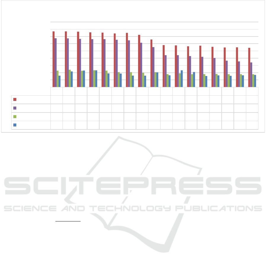
Figure 7: Comparison of Hit rate of alternative TSR algorithms on all four IWSC tasks.

ordering if values are concentrated towards the mid-

range.

Another well performing algorithm is TSR-m,

as given in equation 5, where r is the number of routes

to the target and d is the combined-semantic-distance

of each route. We omit the scaling function for clarity

as it is already given in equation 4. Scaling is applied

once all score values have been calculated.

  







  









(5)

The algorithms TSR-o and TSR-p are the same

as TSR-m except that the exponent of the route’s

rank, which the score is divided by, is 1 and 2

respectively; these variations perform significantly

worse. It is interesting that when penalising the

contribution of additional routes, we see sub-standard

performance when the penalty is small, but above-

standard performance when it is large. This would

suggest that some ideal penalty function exists where

additional routes do not overpower the normal

scoring but still provide support in closely scored

cases. It is possible that the best scoring penalty is a

property of the distribution of the data and labels, and

that the ideal penalty function may be dependent on

the dataset. Testing of this property on other datasets,

and alternative penalties for this dataset are left to

future research.

5.4 Reproducibility

We have made available for download the full suite

of evaluation tools and TSR implementation used in

generating these results, along with the full set of

experimental results and IWSC dataset at

https://github.com/DavidRalph/TSR-Public.

In section 5.3 we describe only the best

performing scoring algorithms. The full

implementation of each can be found in the publicly

available TSR implementation.

6 CONCLUSIONS AND FUTURE

WORK

We have demonstrated the Transitive Semantic

Relationships technique as an effective

recommendation algorithm on datasets with very few

labels and from cold-stats. In particular we see good

performance on the subset-labelling task of the Isle of

Wight Supply Chain dataset also introduced in this

paper. We show that supporting evidence in the form

of additional high-quality routes to a target can have

a positive impact on performance, but that the

weighting used can have a large impact on

performance. Additionally, we find that the inclusion

of additional routes in the scoring can have a negative

effect if the labels are extremely sparse and not

concentrated. Using TSR we set the baseline

performance on the four recommendation tasks for

e m h p a g k l o f n d c q b j i

SL_consumers

0.77 0.77 0.77 0.76 0.75 0.74 0.75 0.72 0.66 0.58 0.58 0.57 0.57 0.56 0.55 0.55 0.54

SL_suppliers

0.68 0.67 0.67 0.66 0.66 0.66 0.65 0.61 0.55 0.44 0.44 0.43 0.42 0.40 0.37 0.36 0.34

ES_consumers

0.23 0.24 0.23 0.23 0.23 0.21 0.21 0.20 0.21 0.18 0.19 0.18 0.18 0.18 0.18 0.18 0.18

ES_suppliers

0.16 0.22 0.23 0.23 0.19 0.19 0.16 0.16 0.20 0.16 0.23 0.21 0.15 0.16 0.16 0.16 0.17

0.00

0.10

0.20

0.30

0.40

0.50

0.60

0.70

0.80

0.90

HR@10

TSR Scoring Algorithm Hit-Rate Comparison

Recommendations from Cold Starts in Big Data

193

the IWSC dataset. Our best performing algorithm

TSR-e showing a hit-rate@10 of 77% on the

SL_consumers task.

The focus of this paper has been on introducing

the TSR technique and IWSC dataset and tasks. Both

contributions open new avenues for further

investigation into the properties of extra sparse, and

subset labelled datasets. Future work could examine

the effects of different embedding models on TSR

and prediction of supply chain competitors and test if

different fine-tuning of these models would further

improve results.

Additional future work could include a

comprehensive analysis of the performance of the

TSR technique on other datasets and how it compares

to or could be used in conjunction with other

recommender systems, particularly as the number of

labels is increased. TSR could also be applied to

expand the number of relationships in a partially

labelled dataset to allow the use of algorithms that

struggle with cold starts or require many training

examples.

REFERENCES

IWChamber (2018). Retrieved from IWChamber:

https://www.iwchamber.co.uk

IWTechnology (2018). Retrieved from IWTechnology:

http://iwtechnology.co.uk/

Marine Southeast (2018). Retrieved from Marine

Southeast: http://www.marinesoutheast.co.uk/

Bowman, S. R., Angeli, G., Potts, C., and Manning, C. D.

(2015). A large annotated corpus for learning natural

language inference. https://doi.org/10.18653/v1/D16-

1264

Cer, D., Yang, Y., Kong, S., Hua, N., Limtiaco, N., John,

R. St., … Kurzweil, R. (2018). Universal Sentence

Encoder. Retrieved from http://

arxiv.org/abs/1803.11175

Grady, C., and Lease, M. (2010). Crowdsourcing

Document Relevance Assessment with Mechanical

Turk, (June), 172–179.

Harper, F. M., and Konstan, J. A. (2015). The MovieLens

Datasets : History and Context r r r, 5(4), 1–19.

He, X., Liao, L., Zhang, H., Nie, L., Hu, X., and Chua, T.-

S. (2017). Neural Collaborative Filtering.

https://doi.org/10.1145/3038912.3052569

Hu, M., and Liu, B. (2004). Mining and summarizing

customer reviews. Proceedings of the 2004 ACM

SIGKDD International Conference on Knowledge

Discovery and Data Mining - KDD ’04, 168.

https://doi.org/10.1145/1014052.1014073

Järvelin, K., and Kekäläinen, J. (2002). Cumulated gain-

based evaluation of IR techniques. ACM Transactions

on Information Systems. https://

doi.org/10.1145/582415.582418

Koren, Y. (2008). Factorization meets the neighborhood: a

multifaceted collaborative filtering model. In

Proceedings of the 14th ACM SIGKDD international

conference on Knowledge discovery and data mining.

https://doi.org/10.1145/1401890.1401944

Maaten, L. Van Der, and Hinton, G. (2008). Visualizing

Data using t-SNE, 9, 2579–2605.

Pang, B., and Lee, L. (2004). A Sentimental Education:

Sentiment Analysis Using Subjectivity Summarization

Based on Minimum Cuts. https://

doi.org/10.3115/1218955.1218990

Snow, R., Connor, B. O., Jurafsky, D., Ng, A. Y., Labs, D.,

and St, C. (2008). Cheap and Fast — But is it Good ?

Evaluating Non-Expert Annotations for Natural

Language Tasks, (October), 254–263.

Suglia, A., Greco, C., Musto, C., De Gemmis, M., Lops, P.,

and Semeraro, G. (2017). A deep architecture for

content-based recommendations exploiting recurrent

neural networks. [UMAP2017]Proceedings of the 25th

Conference on User Modeling, Adaptation and

Personalization, 202–211. https://

doi.org/10.1145/3079628.3079684

Vuurens, J. B. P., Larson, M., and de Vries, A. P. (2016).

Exploring Deep Space: Learning Personalized Ranking

in a Semantic Space. Proceedings of the 1st Workshop

on Deep Learning for Recommender Systems - DLRS

2016, 23–28. https://

doi.org/10.1145/2988450.2988457

Xu, Z., Chen, C., Lukasiewicz, T., Miao, Y., and Meng, X.

(2016). Tag-Aware Personalized Recommendation

Using a Deep-Semantic Similarity Model with

Negative Sampling. Proceedings of the 25th ACM

International on Conference on Information and

Knowledge Management - CIKM ’16.

https://doi.org/10.1145/2983323.2983874

Zhang, F., Yuan, N. J., Lian, D., Xie, X., and Ma, W.-Y.

(2016). Collaborative Knowledge Base Embedding for

Recommender Systems. Proceedings of the 22nd ACM

SIGKDD International Conference on Knowledge

Discovery and Data Mining - KDD ’16, 353–362.

https://doi.org/10.1145/2939672.2939673

IoTBDS 2019 - 4th International Conference on Internet of Things, Big Data and Security

194