Universal Learning Machine with Genetic Programming

Alessandro Re, Leonardo Vanneschi and Mauro Castelli

NOVA Information Management School (NOVA IMS), Universidade Nova de Lisboa,

Campus de Campolide, 1070-312, Lisbon, Portugal

Keywords:

Genetic Programming, Geometric Semantic Genetic Programming, Machine Learning, Ensembles, Master

Algorithm.

Abstract:

This paper presents a proof of concept. It shows that Genetic Programming (GP) can be used as a “universal”

machine learning method, that integrates several different algorithms, improving their accuracy. The system

we propose, called Universal Genetic Programming (UGP) works by deﬁning an initial population of pro-

grams, that contains the models produced by several different machine learning algorithms. The use of elitism

allows UGP to return as a ﬁnal solution the best initial model, in case it is not able to evolve a better one.

The use of genetic operators driven by semantic awareness is likely to improve the initial models, by combin-

ing and mutating them. On three complex real-life problems, we present experimental evidence that UGP is

actually able to improve the models produced by all the studied machine learning algorithms in isolation.

1 INTRODUCTION

According to the No Free Lunch Theorem (Wolpert

and Macready, 1997), if averaged on all existing prob-

lems, all Machine Learning (ML) algorithms have the

same performance. As a consequence, no algorithm

is better than all the others on all existing problems

and so discovering the most appropriate algorithm for

solving one particular application is usually a difﬁ-

cult task. Typically, the choice of the ML technique

involves an experimental comparison between sev-

eral different algorithms. Besides time-consuming,

this experimental phase has also, generally speaking,

an uncertain outcome. In fact, the most appropriate

algorithm for the considered problem may have not

been included in the experimental comparison, or the

results may lack statistical signiﬁcance. This paper

represents the ﬁrst proof of concept that Genetic Pro-

gramming (GP) (Koza, 1992) can be used as a univer-

sal learning machine, able to completely relieve the

user from the choice of the ML algorithm. We do this

by presenting a system, called Universal Genetic Pro-

gramming (UGP), that integrates several different ML

methods, called Basic Learners (BLs), and guarantees

that the returned model is, in the worst case, the best

among the ones generated by the BLs, or hopefully a

signiﬁcant improvement of it.

This is guaranteed thanks to the dynamics of evo-

lution: in UGP the initial population is not random,

as it is usual in GP, but is seeded using the models

returned by the BLs. Such an idea has a major difﬁ-

culty: all the models generated by the BLs should be

represented using the same encoding, and that encod-

ing must be usable by GP (for instance, they should be

represented as trees). This may be very hard to obtain,

given the diverse nature and characteristics of the var-

ious ML algorithms that could be used as BLs. How-

ever, UGP is able to completely avoid this work of

encoding. In fact, UGP uses Geometric Semantic Ge-

netic Programming (GSGP) (Moraglio et al., 2012),

one of the most recent and powerful developments

of GP. GSGP allows us to abstract from the solution

representation since it bases the evolution purely on

semantics. In the GP terminology, semantics is the

vector of outputs of a model on the training obser-

vations. Each model generated by the BLs can be

represented in the UGP population by its semantics.

Hence, it is not needed to carry on its syntactic struc-

ture (that can be extremely large) during the evolu-

tion. In this way, any existing ML algorithm can be

used by UGP as a BL, in a simple way and with no

limitation. GSGP uses Geometric Semantic Opera-

tors (GSOs) instead of the traditional crossover and

mutation. GSOs induce a unimodal error surface (i.e.

a surface with no local optima) for any supervised

learning problem. This fact bestows on UGP the abil-

ity to improve the BLs. Furthermore, UGP counter-

acts overﬁtting, thanks to some well studied theoreti-

cal properties of the GSOs (Vanneschi et al., 2014b).

In this paper, which represents the ﬁrst step in this

Re, A., Vanneschi, L. and Castelli, M.

Universal Learning Machine with Genetic Programming.

DOI: 10.5220/0007808101150122

In Proceedings of the 11th International Joint Conference on Computational Intelligence (IJCCI 2019), pages 115-122

ISBN: 978-989-758-384-1

115

promising research track, only three ML methods are

used as BLs: linear regression, support vector regres-

sion and multi-layer perceptron regression. Further-

more, an extended version of UGP, called UGP with

selection (UGP-SEL), aimed at further counteracting

the overﬁtting of the BLs, is presented. The power of

UGP and UGP-SEL is tested on three real-life sym-

bolic regression problems. Their performance is com-

pared to the one of GSGP and to the one of the BLs

used in isolation.

2 GEOMETRIC SEMANTIC

GENETIC PROGRAMMING

Even though the term semantics can have several dif-

ferent interpretations, it is a common trend in the

Genetic Programming (GP) (Koza, 1992) community

(and this is what we do also here) to identify the se-

mantics of a solution with the vector of its output

values on the training data (Vanneschi et al., 2014a).

Under this perspective, a GP individual can be iden-

tiﬁed with a point (its semantics) in a multidimen-

sional space that we call semantic space. The term

Geometric Semantic Genetic Programming (GSGP)

indicates a recently introduced variant of GP in which

traditional crossover and mutation are replaced by so-

called Geometric Semantic Operators (GSOs), which

exploit semantic awareness and induce precise geo-

metric properties on the semantic space.

GSOs, introduced by Moraglio et al. (Moraglio

et al., 2012), are becoming more and more popular in

the GP community (Vanneschi et al., 2014a) because

of their property of inducing a unimodal error surface

on any problem consisting in matching sets of input

data into known targets (like for instance supervised

learning problems such as regression and classiﬁca-

tion).

In particular

, geometric semantic crossover

generates, as the unique offspring of parents

, T

: R

→ R, the expression:

= (T

· T

) + ((1 − T

) · T

)

where T

is a random real function whose output val-

ues range in the interval [0, 1]. Analogously, geomet-

ric semantic mutation returns, as the result of the mu-

tation of an individual T : R

→ R, the expression:

= T + ms · (T

− T

)

Here we report the deﬁnition of the GSOs as given by

Moraglio et al. for real functions domains, since these are

the operators we will use in the experimental phase. For

applications that consider other types of data, the reader is

referred to (Moraglio et al., 2012).

where T

and T

are random real functions with

codomain in [0, 1] and ms is a parameter called mu-

tation step.

Moraglio et al. (Moraglio et al., 2012) show that

geometric semantic crossover corresponds to geomet-

ric crossover in the semantic space (i.e. the point rep-

resenting the offspring stands on the segment joining

the points representing the parents) and geometric se-

mantic mutation corresponds to ball mutation in the

semantic space (and thus induces a unimodal ﬁtness

landscape on the above mentioned types of problem).

The GSOs implementation presented in (Van-

neschi et al., 2013; Castelli et al., 2015a) not only

makes GSGP usable in practice by solving the draw-

backs pointed out in the original work of Moraglio,

but was also a source of inspiration for the work pre-

sented here. Given that the solutions semantics is

enough to make GSGP work, the population can be

seeded with any solution, even the ones returned by

other ML algorithms. This can be done independently

from the representation used by the ML algorithms

to encode their models. In other words, GSGP al-

lows us to abstract from the representation of the so-

lutions (Moraglio et al., 2012).

GSOs have a known limitation (Vanneschi et al.,

2014a; Castelli et al., 2015a): the reconstruction of

the best individual at the end of a run can be a hard

(and sometimes even impossible) task, due to its large

size. This issue is even more visible in UGP, where

the initial individuals may already be very large (as-

sume for instance that the population is seeded with

a model generated by a deep neural network). This

basically turns UGP into a black-box system.

3 UNIVERSAL GENETIC

PROGRAMMING (UGP)

As mentioned above, GSGP is able to induce a uni-

modal error surface for any supervised learning prob-

lem. Thus, GSGP is characterized by excellent opti-

mization power. Furthermore, solid theoretical foun-

dations (Vanneschi et al., 2013) allow us to state that

GSGP is also able to limit overﬁtting, under some

precise and well-studied circumstances. Taking into

account these characteristics, a new idea comes natu-

rally: seeding the initial population with a set of pre-

dictive models, that have been obtained by as many

ML methods (Basic Learners, BLs), instead of ran-

domly as customary in GP. This is possible and easy,

simply running the BLs, storing the semantics of the

generated models and using them in the initial pop-

ulation of GSGP. GSGP with this new initialization

is called UGP (Universal GP) and presented in this

ECTA 2019 - 11th International Conference on Evolutionary Computation Theory and Applications

116

paper. We can assert that UGP has the following

characteristics: (1) With the simple use of elitism,

well known in GP (Koza, 1992), UGP is able, in the

worst case, to return the best model found by the BLs;

(2) Thanks to the unimodal error surface induced by

GSOs, UGP can easily improve the models found by

the BLs; (3) Thanks to the theoretical properties of

GSGP, UGP is able to limit overﬁtting.

3.1 Universal Genetic Programming

with Selection Mechanism

(UGP-SEL)

The fact that GSGP can limit overﬁtting has been

demonstrated in the literature for a traditional ran-

domly generated initial population (Castelli et al.,

2014b). When, as it is the case for UGP, the initial

population integrates randomly generated individuals

with models that have already been trained (the mod-

els generated by the BLs), the picture can be differ-

ent. Indeed, it is expected that the models generated

by the BLs will have a much better training ﬁtness

than the randomly generated ones, and thus they will

be selected for mating many times, at least in the ﬁrst

phase of the evolution. In such a situation, it is easy

to imagine that if those models overﬁt training data, it

will be very hard for UGP to return a ﬁnal model that

does not overﬁt. In simple words, we have to avoid to

seed the population with overﬁtting models.

The objective of UGP-SEL is to minimize the

possibility of having overﬁtted models in the initial

population. This is obtained by means of a pre-

evolutionary selection procedure aimed at estimating

the generalization ability of BLs before adding them

to the initial population. This is done using a val-

idation dataset which is separated from the dataset

used for training the BLs. The selection procedure we

introduce works by partitioning the entire dataset in

three subsets: training, validation and testing datasets.

The training dataset is used to train the BLs. The

validation is used to estimate the performance of the

models generated by the BLs, with the objective of

discarding the overﬁtting ones. Training can then

take place again using both the training and validation

datasets. The output performances are then measured

on the testing dataset, which is completely unknown

to the models. In this scheme, different selection pro-

cedures can be adopted, for example discarding BLs

that have excessively poor validation performance

when compared to training. This procedure scales

well with the number of models used to construct the

BLs, as it requires a single training and a single val-

idation for each learner, and can be adopted once a

strategy for evaluating the performance and discard-

ing BLs is deﬁned. In our case, to obtain robust

statistical evidence, we adopt a nested K-fold cross-

validation procedure, which involves testing which

combination of models yields the best performance

after a short run of UGP. The winning combination of

models is then used for a long run of UGP.

More precisely, let D be the entire dataset and p

its i-th partition. Then, in K-fold cross-validation, the

datasets used in the k-th fold are deﬁned as d

= p

and d

= D \ p

, for 1 ≤ k ≤ K. Similarly, we perform

nested J-fold cross-validation by deﬁning the datasets

k j

and n

k j

, obtained by partitioning d

instead of D ,

having n

k j

∪ n

k j

= d

for 1 ≤ j ≤ J. Given a set of

M models generated by the BLs, the pre-evolutionary

selection procedure we used ﬁrst involved training all

the models over n

k j

, then take every combination of

models and performing a short UGP run, using the

same dataset n

k j

to compute ﬁtness values, and eval-

uating their performances over n

k j

. The results of

these runs are averaged across the J-folds, and the

best combination of models is selected to be used in

the next phase. Once a combination of models is se-

lected, it is used to perform a long run of UGP: mod-

els are trained again over d

, which is also used to

compute the ﬁtness during the evolution, while d

used for evaluation purposes (test set). Note that this

procedure is repeated K times and then averaged.

UGP-SEL, as we deﬁned it, is computationally ex-

pensive: it requires to train models multiple times

over different datasets, suffers from a combinatorial

explosion when M increases and requires to execute

a large number of (short) UGP runs. However, the use

of UGP-SEL gave us some useful insights, as it will

appear clear when we will present our experimental

study (Section 4).

4 EXPERIMENTAL STUDY

4.1 Test Problems and Experimental

Settings

For each model, 60 runs were performed adopting a 5-

fold cross-validation scheme and, where applicable, a

nested 4-fold cross-validation. Each run used a popu-

lation of 200 individuals and a total of 200000 ﬁtness

evaluations were performed. When UGP-SEL was

used, the brief evolutionary stage consisted of 4000

ﬁtness evaluations. The population was initialized

with the ramped half and half method (Koza, 1992),

except for UGP, where the population is seeded us-

ing the three models evolved by Multilayer Percep-

tron, Support Vector Regression and Linear Regres-

Universal Learning Machine with Genetic Programming

117

sion, while the remaining 197 individuals are initial-

ized using the ramped half and half algorithm, with

an initial maximum height of 6. No height constraints

were in place after initialization. For UGP-SEL the

initialization is done using the models chosen by the

selection mechanism described in Section 3.1, plus

the remaining individuals generated randomly using

ramped half and half. Besides those parameters, the

primitive operators were addition, subtraction, multi-

plication, and division protected as in (Koza, 1992).

The terminal symbols included one variable for each

feature in the dataset and no constants. Parent selec-

tion was done using tournaments of size 4. Crossover

rate and mutation rate were equal to 70% and 30%

respectively. These values were selected after a pre-

liminary tuning phase aimed at discovering the most

suitable values of the parameters, and since a manual

tuning of the parameters showed no (statistically sig-

niﬁcant) difference in terms of performance with re-

spect to other conﬁgurations tested. This is related to

the fact that it has become increasingly clear that GP

is very robust to parameter values once a good conﬁg-

uration is determined, as suggested by a recent large

and conclusive study (Sipper et al., 2018). The error

measure adopted to measure the ﬁtness of one seman-

tic against the train semantic was the Mean Absolute

Error (MAE).

Table 1: Description of the test problems. For each dataset,

the number of features and the number of instances are re-

ported.

Dataset # Features # Instances

Parkinson (Castelli

et al., 2014a)

26 5875

Energy (Castelli

et al., 2015b)

8 768

Concrete (Castelli

et al., 2013)

8 1029

The test problems that we have used in our ex-

perimental study are three symbolic regression real-

life applications. The ﬁrst one (Parkinson) aims at

predicting the value of the uniﬁed Parkinson’s dis-

ease rating scale as a function of several patients fea-

tures, mainly extracted from their voice. The sec-

ond problem (Energy) has the objective of forecasting

the value of the energy consumption in some particu-

lar geographic areas and on some particular days, as

a function of some of the observable characteristics

of that (and previous) day(s) (for instance meteoro-

logic characteristics and others). Finally, the Concrete

problem aims at predicting the value of the concrete

strength, as a function of some features of the mate-

rial. All these problems have already been used in

previous GP studies (Castelli et al., 2014b; Castelli

et al., 2014a; Castelli et al., 2013; Castelli et al.,

2015b). Table 1 reports, for each dataset, the num-

ber of features (variables) and the number of instances

(observations). For a complete description of these

datasets, the reader is referred to the references re-

ported in the same table.

4.2 Experimental Results

The experimental study aims at understanding the

real advantage of using GP as a universal learning

method. To accomplish this task, we analyzed differ-

ent aspects. We initially compared the performance

over training and unseen instances of three different

GP-systems: GSGP, UGP, and UGP-SEL. The re-

sults of this analysis are reported in Figure 1. Fo-

cusing on the performance achieved on the training

instances, and considering the three benchmark prob-

lems, it is possible to observe a common trend: UGP

and UGP-SEL produce results that are comparable

between each other and outperform GSGP on all the

studied test problems. Interestingly, the models pro-

duced by the BLs are effectively improved in the evo-

lutionary process. In fact, both UGP and UGP-SEL

have steady improvement in terms of ﬁtness during

the whole evolution. Additionally, UGP-SEL is able

to reduce the computational time needed for obtain-

ing good quality models for the Energy benchmark.

Hence, the selection of the best models produced by

the BLs, that is typical of UGP-SEL, is not detrimen-

tal and, on the contrary, can speed up the search pro-

cess for some problems. Also, GSGP produces a stan-

dard deviation (grey area surrounding the GSGP line

in the plots) that, while presenting an acceptable mag-

nitude, is larger than the one produced by UGP and

UGP-SEL. We conclude that using GP for evolving

models obtained from other ML techniques provides

a beneﬁcial effect on the ﬁnal model, that is character-

ized by a lower error and a lower standard deviation

with respect to the one produced by GSGP.

While results achieved on the training instances

are important, the performance on the test set is a

fundamental indicator to assess the robustness of the

model with respect to its ability in generalizing over

unseen data. This is a property that must be ensured

in order to use an ML technique for addressing a real-

world problem. As one can observe from Figure 1, in

all the considered benchmarks, UGP and UGP-SEL

are able to generalize well over unseen instances, out-

performing GSGP on all the studied problems. Also

on the test set, UGP and UGP-SEL are able to im-

prove the performance of the models produced by the

BLs and, even more interesting, are able to combine

ECTA 2019 - 11th International Conference on Evolutionary Computation Theory and Applications

118

(a) (b) (c)

(d) (e) (f)

Figure 1: Results on training (a,c,e) and test sets (b,d,f). Median over 30 runs. Plot (a,b): Energy dataset.

Plot (c,d): Concrete dataset. Plot (e,f): Parkinson dataset.

these models for obtaining a ﬁnal solution that corre-

sponds to a ”blend” of different ML techniques. The

ﬁnal solution produces good performance over the

training data as well as a good generalization ability

and it is characterized by a lower standard deviation

with respect to GSGP. All in all, the idea of using GP

as a universal learning method seems very promising.

To assess the statistical signiﬁcance of the results

presented in Figure 1, a statistical validation was per-

formed. First of all, given it is not possible to as-

sume a normal distribution of the values obtained by

running the different techniques, we ran the Lilliefors

test, using α = 0.05. The null hypothesis of this test is

that the values are normally distributed. The result of

the test suggests that the null hypothesis should be re-

jected. Hence, we used the Mann-Whitney U test for

comparing the results returned by the different tech-

niques considered under the null hypothesis that the

distributions are the same across repeated measures.

Also in this test, a value of α = 0.05 was used and

the Bonferroni correction was considered. Table 2 re-

ports the p-values returned by the Mann-Whitney test.

A bold font is used to denote values suggesting that

the alternative hypotheses cannot be rejected (statisti-

cally signiﬁcant results). According to this study, for

all the studied benchmarks, UGP and UGP-SEL ob-

tained models that are better (i.e., with lower error)

than the ones produced by GSGP and the differences

in terms of error are statistically signiﬁcant on both

training and test data.

To gain a full comprehension of the dynamics of

UGP, the second part of the experimental phase ana-

lyzes the contribution provided by the different BLs

in the construction of the ﬁnal model. The objective

is to understand what are the sub-components of the

ﬁnal solution that were formed thanks to a blend of

different ML techniques. To answer this question, we

Table 2: P-values returned by the Mann-Whitney test for

the benchmarks considered. Bold values used to denote sta-

tistically signiﬁcant results.

Energy

Training Test

UGP UGP-

SEL

UGP UGP-

SEL

GSGP 3.6E-21 3.6E-21 3.6E-21 3.6E-21

UGP - 4.4E-21 - 3.2E-12

Concrete

Training Test

UGP UGP-

SEL

UGP UGP-

SEL

GSGP 3.6E-21 3.6E-21 3.6E-21 3.6E-21

UGP - 0.52 - 0.53

Parkinson

Training Test

UGP UGP-

SEL

UGP UGP-

SEL

GSGP 3.6E-21 3.6E-21 3.6E-21 3.6E-21

UGP - 0.27 - 0.04

perform the following analysis: we associate to each

candidate solution a vector, whose length is equal to

the number of used BLs, plus one. Each component

of this vector will be associated with a different BL,

and the further component will be associated to GP.

For all the individuals initialized randomly (with the

ramped-half-and-half technique in our case), the po-

sition of the vector corresponding to GP is initialized

with a value equal to 1, while all the other positions

are initialized with a value equal to 0. For each model

generated by a BL, the vector is initialized with a

value equal to 1 in the position corresponding to that

BL, and 0s in all other positions. After each crossover

Universal Learning Machine with Genetic Programming

119

event, we summed up the vectors of the parents to ob-

tain a new vector that can, in some senses, be inter-

preted as the “ﬁngerprint” of the child. In this way,

at the end of the evolutionary process, we are able to

quantify the contribution of each BL and of GP itself

to the construction of the ﬁnal solution. Theoretically,

an individual that has a value equal to the number of

crossover events in the position of the vector corre-

sponding to GP, and a value equal to 0 is all other

positions is a model that has been generated purely

by GP, without any contribution from any of the BLs.

On the other hand, the values in the positions corre-

sponding to the BLs quantify the contribution of the

various BLs in the formation of that individual. The

results of this analysis are reported in Figure 2 and

in Figure 3, where the values contained in the vec-

tor associated to the best individual at the end of the

evolution are reported, after having been normalized

in a [0, 1] scale. Figure 2 reports the results for UGP,

while Figure 3 shows the analogous results for UGP-

SEL.

The ﬁrst important observation is that none of

the best-evolved models (neither the ones evolved by

UGP nor the ones evolved by UGP-SEL) is a purely

GP-evolved individual. All of them have an impor-

tant contribution by the BLs. Furthermore, only in

one case, the ﬁnal model is formed by a 100% contri-

bution from only one BL. It is the case of UGP-SEL

in the Energy dataset, reported in Figure 3(a), where

the ﬁnal model was formed by a 100% contribution of

SVR. In all other cases, the ﬁnal model is formed by

a blend between different BLs and GP. Before contin-

uing with the analysis of Figures 2 and 3, it is impor-

tant to point out that if an individual is formed by a

100% contribution of one BL, this does not necessar-

ily mean that the ﬁnal model was the one generated by

that BL, and used to initialize the GP population. In-

deed, in GP it is possible to have a crossover between

one individual and itself, and when GSOs are used

(as in this work), the offspring is an individual that is

very different from the parent. Indeed, what happened

with UGP-SEL in the case of the Energy dataset (Fig-

ure 3(a)) is that the ﬁnal model was obtained by vari-

ous crossovers between individuals that, although dif-

ferent between each other, are all descendants from

the model generated by SVR. This is proven by the

fact that the curve of the evolution of UGP-SEL for

this problem is not constant (see Figure 1(a)), but the

error is steadily decreasing along with the evolution.

Thus, the ﬁnal model is not the one generated by SVR

and used in the initialization, but an improvement of

it.

Analyzing Figures 2 and 3 more in detail, one

can remark that on the Energy dataset the ﬁnal model

was only inﬂuenced by SVR in the case of UGP-SEL

(Figure 3(a)), while the best solution is obtained by

a blend of LR and SVR in the case of UGP (Fig-

ure 2(a)). In the latter case, the model consists of a

contribution of 98% given by LR and the remaining

2% by SVR. Looking back at Figure 1, it is interesting

to notice that while UGP and UGP-SEL performed

in a comparable manner, the best solutions they pro-

duced have been formed by combining different BLs.

This observation further corroborates the importance

of semantics: despite the solutions having completely

different structures, because they are formed by re-

combinations of models generated by different BLs,

they have a similar behaviour, that is what matters for

assessing the models’ performance. Taking into ac-

count the Concrete dataset, it is possible to see that the

ﬁnal model of UGP (Figure 2(b)) was generated using

a contribution of approximately 40% of GP, 35% of

LR, 20% of MLP, and 5% of SVR. On the same prob-

lem UGP-SEL (Figure 2(c)) behaves similarly but,

with respect to UGP, a more important contribution

to the construction of the best model is given by GP

and LR, while MLP and SVR decreased their con-

tribution. Finally, on the Parkinson benchmark, we

have a similar situation where both UGP and UGP-

SEL built a ﬁnal model with a contribution of approx-

imately 55% of SVR, 30% of GP, 10% of LR, and 5%

of MLP (Figures 2(e) and 2(f)).

To conclude the experimental study, we focused

on UGP-SEL and we analyzed the number of times in

which the model generated by a BL was selected to

be inserted in the initial population, using the selec-

tion process described in Section 3.1. This analysis is

reported in Figure 4.

Remembering that each one of the independent

runs that we have performed uses a different train-

ing/test partition of the data, and thus also the ini-

tial models generated by the BLs are different be-

tween each other in the different runs, we can ob-

serve that for the Energy problem (Figure 4(a)), in

more than 60% of the runs both the models generated

by LR and SVR are inserted in the initial population,

while in the remaining runs only the model generated

by SVR was selected and inserted in the initial popu-

lation. On the Concrete dataset (Figure 4(b)), in more

than 40% of the runs all the studied BL models (SVR,

LR and MLP) were selected to be part of the initial

population, and in more than 30% of the runs the

models that were selected and inserted in the initial

population were the ones generated by LR and MLP.

Looking back at the results of Figure 3, we can see

that the evolutionary process is able to combine the

solutions composed by the aforementioned BLs, im-

proving them; but, despite that, the ﬁnal model was

ECTA 2019 - 11th International Conference on Evolutionary Computation Theory and Applications

120

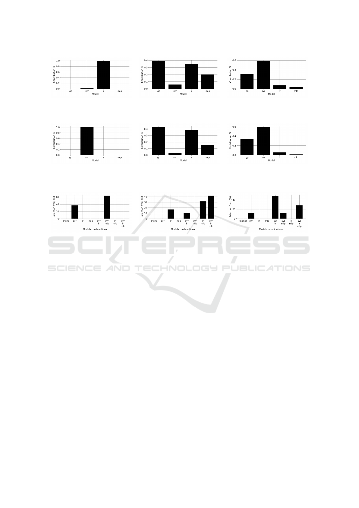
(a) (b) (c)

Figure 2: Percentage contribution provided by the different BLs for building the best ﬁnal model for UGP.

Plot (a): Energy dataset. Plot (b): Concrete dataset. Plot (c): Parkinson dataset.

(a) (b) (c)

Figure 3: Percentage contribution provided by the different BLs for building the best ﬁnal model for UGP-SEL.

Plot (a): Energy dataset. Plot (b): Concrete dataset. Plot (c): Parkinson dataset.

(a) (b) (c)

Figure 4: Techniques that provided the best model after the initial selection phase. Plot (a): Energy dataset.

Plot (b): Concrete dataset. Plot (c): Parkinson dataset.

built also with a 40% contribution of GP. Hence,

also for the Concrete dataset, the evolutionary process

seems to be able to improve the performance of “sim-

ple” models (i.e. generated with the contribution of

only one technique) more easily with respect to “hy-

brid” models (i.e. formed thanks to a blend of more

than one technique). Finally, Figure 4(c) presents the

results obtained on the Parkinson dataset. In this case,

we can observe that the models generated by SVR are

always selected to be inserted in the initial population.

More than 40% of the times, the models that are in-

serted in the initial population are the one generated

by SVR and the one generated by LR, while approx-

imately 30% of the times the models inserted in the

initial population are the ones generated by the three

studied BLs (i.e. SVR, LR, and MLP). This result is

consistent with the one reported in Figure 3(f), where

the most important contribution for the construction

of the ﬁnal best model for this problem is provided by

SVR. Anyway, also for this dataset, an important con-

tribution to the ﬁnal model is provided by GP itself.

This observation strengthens the previous conjecture:

for GP, improving “simple” models is easier than im-

proving “hybrid” ones. In conclusion, the experimen-

tal study allowed us to discover interesting insights

about UGP and UGP-SEL. In particular, UGP and

UGP-SEL behave similarly to ensemble techniques

for their ability in producing robust models, as well

as reducing the variance bias. Additionally, the best

model returned by both UGP and UGP-SEL always

consists of a composition of different contributions

from more than one ML technique.

5 CONCLUSIONS AND FUTURE

WORK

The objective of this paper was to present a proof of

concept, and the paper was conceived as a beginning

step in a long and promising research track. The sci-

entiﬁc question behind this work is if Genetic Pro-

gramming (GP) can be used as a “universal” Ma-

chine Learning (ML) system. In this context, with

the term universal, we mean a system able to join

several (and potentially even all existing) ML algo-

rithms (called Basic Learners – BLs –), and, in the

worst case, always return the best model generated by

any of these algorithms. The idea developed in this

work consists of using several ML models to seed

Universal Learning Machine with Genetic Programming

121

a GP population. The major obstacle to this idea is

bound to representation: all the used models should

employ the same representation, and this representa-

tion should be “usable” by GP. This obstacle is by-

passed by the use of Geometric Semantic GP (GSGP),

that is able to completely abstract from the represen-

tation. These ideas have been implemented in two

systems that were presented in this paper: a ﬁrst sys-

tem called Universal GP (UGP), and its variant, called

selective UGP (UGP-SEL), where only a subset of the

models generated by the BLs are selected and retained

in the initial population, in order to limit overﬁtting.

The suitability of UGP and UGP-SEL has been tested

on three real-life symbolic regression problems. UGP

and UGP-SEL have been compared with GSGP and

the BLs themselves, that in this preliminary work

were linear regression, support vector regression and

multi-layer Perceptron. UGP and UGP-SEL have

clearly outperformed all these methods in a statisti-

cally signiﬁcant way. Furthermore, our experimental

study has clearly shown that the ﬁnal models returned

by UGP and UGP-SEL are often obtained by a blend

of different models generated by different ML algo-

rithms.

In spite of the very promising results presented in

this paper, the work is still in an initial phase, and

a lot of work is expected in the near future. First,

given that this work was just intended as a ﬁrst proof

of concept, only three BLs were used so far. On the

other hand, in order to exploit the potentiality of the

idea, many different BLs have to be used. Also, better

ways of joining the models generated by the BLs, by

means of speciﬁc and new types of crossover, deserve

investigation.

ACKNOWLEDGMENT

This work was supported by national funds through

FCT (Fundac¸

ao para a Ci

encia e a Tecnologia) un-

der project DSAIPA/DS/0022/2018 (GADgET) and

project PTDC/CCI-INF/29168/2017 (BINDER).

Mauro Castelli acknowledges the ﬁnancial support

from the Slovenian Research Agency (research core

funding No. P5-0410).

REFERENCES

Castelli, M., Silva, S., and Vanneschi, L. (2015a). A

c++ framework for geometric semantic genetic pro-

gramming. Genetic Programming and Evolvable Ma-

chines, 16(1):73–81.

Castelli, M., Trujillo, L., Vanneschi, L., and Popovi

c, A.

(2015b). Prediction of energy performance of resi-

dential buildings: A genetic programming approach.

Energy and Buildings, 102:67 – 74.

Castelli, M., Vanneschi, L., and Silva, S. (2013). Prediction

of high performance concrete strength using genetic

programming with geometric semantic genetic opera-

tors. Expert Systems with Applications, 40(17):6856 –

6862.

Castelli, M., Vanneschi, L., and Silva, S. (2014a). Predic-

tion of the uniﬁed parkinson’s disease rating scale as-

sessment using a genetic programming system with

geometric semantic genetic operators. Expert Systems

with Applications, 41(10):4608 – 4616.

Castelli, M., Vanneschi, L., Silva, S., and Ruberto, S.

(2014b). How to exploit alignment in the error space:

Two different gp models. In Genetic Programming

Theory and Practice XII, Genetic and Evolutionary

Computation, pages 133–148, Ann Arbor, USA.

Koza, J. R. (1992). Genetic Programming: On the Pro-

gramming of Computers by Means of Natural Selec-

tion. MIT Press, Cambridge, MA, USA.

Moraglio, A., Krawiec, K., and Johnson, C. (2012). Ge-

ometric semantic genetic programming. In Parallel

Problem Solving from Nature - PPSN XII, volume

7491 of Lecture Notes in Computer Science, pages

21–31. Springer Berlin Heidelberg.

Sipper, M., Fu, W., Ahuja, K., and Moore, J. H. (2018).

Investigating the parameter space of evolutionary al-

gorithms. BioData Mining, 11(1):2.

Vanneschi, L., Castelli, M., Manzoni, L., and Silva, S.

(2013). A new implementation of geometric seman-

tic GP and its application to problems in pharmacoki-

netics. In Proceedings of the 16th European Con-

ference on Genetic Programming, EuroGP 2013, vol-

ume 7831 of LNCS, pages 205–216, Vienna, Austria.

Springer Verlag.

Vanneschi, L., Castelli, M., and Silva, S. (2014a). A survey

of semantic methods in genetic programming. Genetic

Programming and Evolvable Machines, pages 1–20.

Vanneschi, L., Silva, S., Castelli, M., and Manzoni, L.

(2014b). Geometric semantic genetic programming

for real life applications. In Genetic Programming

Theory and Practice XI, pages 191–209. Springer

New York.

Wolpert, D. H. and Macready, W. G. (1997). No free

lunch theorems for optimization. Trans. Evol. Comp ,

1(1):67–82.

ECTA 2019 - 11th International Conference on Evolutionary Computation Theory and Applications

122