
Camera and Lidar Cooperation for 3D Feature Extraction
Burtin Gabriel
1
, Bonnin Patrick
2
and Malartre Florent
1
1
4D-Virtualiz, 10 Allee Evariste Galois, Clermont-Ferrand, France
2
LISV, Universite de Versailles St Quentin, 10-12 Avenue de l’Europe Velizy, France
Keywords:
Line Segment Detection, Algorithm Optimization, Camera-lidar Sensor Fusion, Localization, Extended
Kalman Filter.
Abstract:
The objective of this work is to use efficiently various sensors to create a SLAM system. This algorithm
has to be fast (real-time), computationally light and efficient enough to allow the robot to navigate in the
environment. Because other processes embedded require large amount of cpu-time, our objective was to use
efficiently complementary sensors to obtain a fairly accurate localization with minimal computation. To reach
this, we used a combination of two sensors: a 2D lidar and a camera, mounted above each other on the robot
and oriented toward the same direction. The objective is to pinpoint and cross features in the camera and
lidar FOV. Our optimized algorithms are based on segments detection. We decided to observe intersections
between vertical lines seen with the camera and locate them in 3D with the ranges provided by the 2D lidar.
First we implemented a RGB vertical line detector using RGB gradient and linking process, then a lidar data
segmentation with accelerated computation and finally we used this feature detector in a Kalman filter. The
final code is evaluated and validated using an advanced real-time robotic simulator and later confirmed with a
real experiment.
1 INTRODUCTION
The robot of the future is built to work in the new
hi-tech ”factory”. It is given tasks to complete in
a cluttered, yet structured and human environment.
To complete these tasks, the robot must move be-
tween locations, with a possibility of encountering
humans. We need a navigation system to able to
work fast, be reliable and take advantage of the struc-
tured characteristic of the environment. This problem
can be divided in sub-tasks: localization, mapping,
path-planning, control and safety management. All
these tasks must be performed within an embedded
computation unit on the robot. This means that each
task must consume computational resources as little
as possible. On the other hand, the robot is moving
and needs a regular update on its status. The goal is
to reduce computation cost induced by each element
of the navigation system. The concept of localiza-
tion is to give the robot an idea of ”where” it is on
a map. This map can be either known previously or
built during the robot evolution in the environment,
also known as SLAM (simultaneous localization and
mapping (Durrant-Whyte and Bailey, 2006)).
In our case, the environment is human made, com-
posed of a flat floor, rooms with various sizes, shapes
and furniture, all of them connected though hallways.
This environment is likely to be an hospital, a factory
or offices, thus it is populated and traveled by humans
at all times. The place is neither collaborative (we
don’t use man-made landmarks) nor hostile (nothing
is going to make an attempt at putting the robot out of
action). Humans are considered as ”passive” distur-
bance and are not likely actively trying to break the
robot. Human detection and handling have yet to be
done but are not part of this work; however, they have
direct effects on the degrees of freedom. These two
steps are indeed achieved through the analysis of sen-
sor data provided by a camera. As we can see, one
sensor is already decided. This human detection pro-
cess is particularly CPU-consuming and have priority
(safety is the most important task), therefore, the CPU
time allowed to our algorithm is reduced. This low-
ered CPU time availability is a major constraint to be
taken into account in the design of our localization
method.
First we will have a look at previous and related
work, then we will detail the vision and lidar process
followed by an implementation of this feature extrac-
tor in a SLAM algorithm using an Extended Kalman
Gabriel, B., Patrick, B. and Florent, M.
Camera and Lidar Cooperation for 3D Feature Extraction.
DOI: 10.5220/0007808900230033
In Proceedings of the 16th International Conference on Informatics in Control, Automation and Robotics (ICINCO 2019), pages 23-33
ISBN: 978-989-758-380-3
Copyright
c
2019 by SCITEPRESS – Science and Technology Publications, Lda. All rights reserved
23

Filter. At last, the performances are first evaluated us-
ing an advanced real-time robotic simulator (Burtin
et al., 2016), then with a real robot/sensor set-up.
2 RELATED WORK
Using segments to perform SLAM processing have
been explored either with a lone lidar (Roumelio-
tis and Bekey, 2000), (Choi et al., 2008) or camera
alone (Huang, 2008), (Lemaire and Lacroix, 2007),
(Micusik and Wildenauer, 2015), (Zuo et al., 2017).
SLAMs are generally split between sparse and dense
vision algorithms. Sparse SLAMs are using only a
few salient features in the image to compute the lo-
calization, for example the ORB-SLAM (Mur-Artal
et al., 2015). Each feature is represented and stored
specifically in the map to be used later as reference
in the localization algorithm. These types of process
only need a small percentage of the pixels from the
entire image to be tracked, while dense methods use
almost all the pixels. Because dense methods such
as DTAM (Newcombe et al., 2011) uses every pixels
from the image, users need a powerful hardware to
perform all the operations in real-time. Most of the
time, GPU processing is used to improve the compu-
tation speed. RGB-D (Kinect, Xtion) and depth cam-
era sensors brought new SLAMs systems (Engelhard
et al., 2011), (Schramm et al., 2018), with new ap-
proaches. They avoid the issue of initialization from
unknown range for the features. Monocular cameras
have the weakness to be unable, using only one frame,
to obtain the distance between an object and the cam-
era for its given pixel in the image (scale effect). LSD
(Von Gioi et al., 2012) is massively used by monoc-
ular and stereo-vision SLAMs systems (Engel et al.,
2014) or (Pumarola et al., 2017) but this line segment
detector is too generic and extracts all segments avail-
able while processing only B&W images: the pro-
cess is not optimized enough. Moreover, the RGB to
B&W conversion is a potential danger of missing gra-
dients because of the gray level conversion method.
The idea to use both lidar and monocular camera has
been more usually applied to mobile objects detec-
tion and tracking (Premebida et al., 2007), (Asvadi
et al., 2016), (De Silva et al., 2018) but more rarely
to localization itself. In our case, we will focus on
the detection of vertical lines in the camera because
they are commonly found and invariants regarding our
environment. The common slam, using these types
of features are commonly referred as ”bearing” only
slam (Bekris et al., 2006), they are proven effective in
minimalist set-ups with simple environments (Huang,
2008), (Choi et al., 2008), (Zuo et al., 2017).
In order to extract these vertical segments in the
image (which are supposed to be the projection of 3D
vertical structures of the scene: doors, angles of corri-
dors), we are looking for classical edge segmentation
composed of well known steps (Nachar et al., 2014):
1. gradient computation ;
2. thinning ;
3. closing ;
4. linking ;
5. and polygonal approximation.
The gradient computation being the most time
consuming step, we will detail the choice of the
appropriate algorithm in this section, its adaptation
and its time optimized implementation (Cabrol et al.,
2005) in the next section.
The gradient computation algorithms could be
classified into three categories, according to their
complexity, and the size of the neighborhood:
• 2 × 2: Roberts (Roberts, 1965) proposed in the
60’s;
• 3 × 3: Prewitt (Prewitt, 1970), Sobel (Sobel,
1978) and Kirsh (Kirsch, 1971) in the 70’s;
• JF Canny ((Canny, 1983)) (in OpenCV),
R.Deriche ((Deriche, 1987)) in the 80’s.
Although better quality results are obtained by algo-
rithms of the last category, the best compromise be-
tween the quality of results and the sum of computa-
tions, for our real-time and embedded robotic appli-
cation, is given by the second one.
The principle of Prewitt and Sobel algorithms is to
compute the projection of the gradient
−→
G on the axis
of the image:
−→
u
x
and
−→
u
y
first and, then, to perform a
rectangular to polar transformation to obtain:
• the gradient magnitude, which is the reflect of the
transition between two regions;
• the gradient argument, which is orthogonal to the
local edge direction. This information is reduced
to the knowledge of direction of the neighbor
pixel in the orthogonal direction of the edge for
the thinning step, ie. four directions.
||
−→
G || =
q
(
−→
G .
−→
u
x
)
2
+ (
−→
G .
−→
u
y
)
2
Arg(
−→
G ) = arctan
−→
G .
−→
u
y
−→
G .
−→
u
x
!
In order to obtain quite same results, and avoid
the computations (in double floats if done without ap-
proximation) of the rectangular to polar transform,
Kirh introduced two diagonal direction of projection:
ICINCO 2019 - 16th International Conference on Informatics in Control, Automation and Robotics
24
−→
u
45
and
−−→
u
−45
. Thus the gradient magnitude was ap-
proximated by the longer projection, and the argu-
ment by the Freeman code corresponding to the best
projection.
||
−→
G || = Max{|
−→
G .
−→
u
x
|,|
−→
G .
−→
u
y
|,|
−→
G .
−→
u
45
|,|
−→
G .
−−→
u
−45
|}
Arg(
~
G) =
0, if ||
−→
G || = |
−→
G .
−→
u
x
|
6, if ||
−→
G || = |
−→
G .
−→
u
y
|
1, if ||
−→
G || = |
−→
G .
−→
u
45
|
7, if ||
−→
G || = |
−→
G .
−−→
u
−45
|
Another way, which seems to be promising, is to
use Edgels or Line Segment Detectors: small edge
segments are gathered into bigger ones using region
growing algorithms.
3 APPROACH
The most important statement considering our hy-
pothesis is the fact that the robot is evolving in a
man-made environment, comparable to an industry
(factory) or office/hospital type. We state that the
robot will encounter numerous structured elements
with strong vertical and horizontal lines. Consider-
ing a flat floor, we also assume that the movement
is only 2D. With this new assumption and the previ-
ous one, we can narrow features to propose a sparse
localization method using specific landmarks. The
most invariant observable elements in the image, as
explained before, are going to be the vertical lines. 3D
horizontal and other more random lines would have
an incidence angle due to the point of view of the
camera and wouldn’t be invariant in the image, thus
inducing more computation to detect and track them.
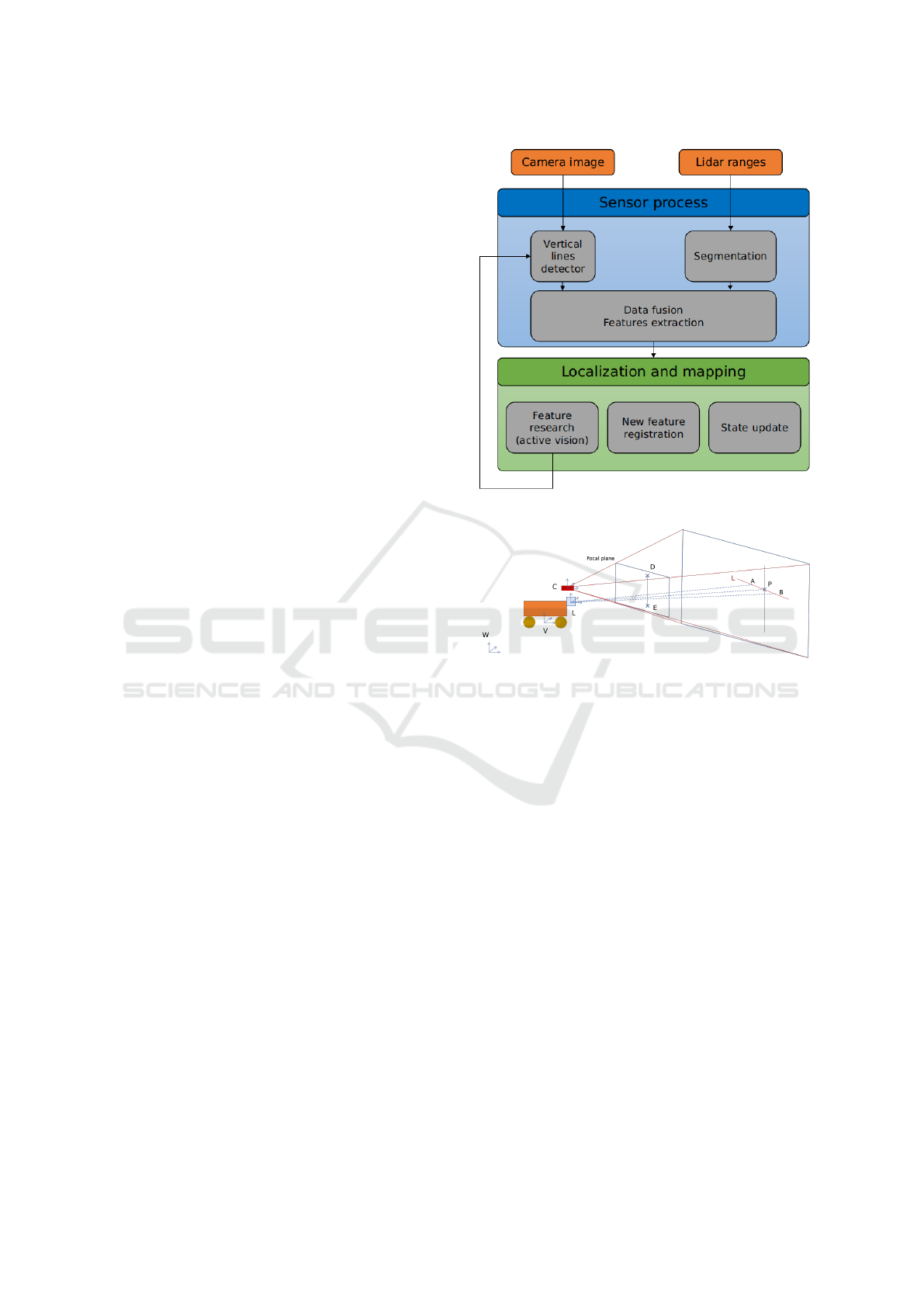
The localization process is an optimized parallel
pipeline able to cross data from the lidar and camera
sensors (Figure: 1). Each data process is split, but
synchronous to use both extracted data at the same
moment during the feature extraction stage. The ob-
jective is to detect a feature and determine its 3D po-
sition in the camera frame. The camera process ex-
tracts vertical lines in the image while the lidar pro-
cess does a segmentation and a time-forward predic-
tion to match the camera’s data time-stamp.
The lidar, placed horizontally on the robot, pro-
duces an horizontal plane with the successive dis-
tances measurements. Our lidar process produces,
through the lidar segmentation algorithm, a set of
lines representing the environment around our robot.
The camera, located above the lidar, through the lines
detection algorithm, extracts a set of vertical lines in
the focal plane of the image. The fusion of both of
these data gives us a set of 3D points in the camera
frame (Figure: 2).
Figure 1: System overview.
Figure 2: Feature (P) detected in the focal and lidar plane.
First we will see the optimized vertical lines de-
tection algorithm for images processing.
Then we will develop the 3D points extraction
process using the camera vertical features and the hor-
izontal lines from the lidar process.
In the end, we will propose a SLAM implemen-
tation using the extracted features from the previous
processes.
3.1 Vision Process
Our goal is to extract vertical segments for a real time
vision system on a small robot. Although general pur-
pose edge detectors exist, and we implement several
kinds by ourselves (Cabrol et al., 2005), they are not
optimal in our particular case.
If we refer to the quicker general purpose method
proposed by Kirsh, the use of the horizontal mask
which detects horizontal gradient ie. local vertical
edge, is sufficient. This simple remark allows to di-
vide by more than four (one mask compared to four
masks computation and the selection) the required
computing time.
In the same manner all the following steps: thin-
Camera and Lidar Cooperation for 3D Feature Extraction
25
ning, closing, linking, and polygonal approximation
are simplified (Nachar et al., 2014), and could be run
faster:
• for the thinning step: only the horizontal left
neighbor pixel is considered;
• for the closing step: only the one vertical neigh-
bor, depending on the direction of the edge is re-
cursively followed;
• for the polygonal approximation: this step is
wholly simplified, because only vertical segments
are taken into account. There is only one vertical
segment by edge, so there is no need to compute
a distance between the edge and the segment in
order to cut the edge into several segments consti-
tuting the polygonal line.
The adaptation from B&W to RGB edge segmen-
tation which is not available on OpenCV is trivial.
However, there are in images a lot of chrominance
edges, that is to say edges between regions from dif-
ferent colors with the same luminance, which are im-
possible to extract using B&W edge segmentations.
Starting from the following observation, a chromi-
nance edge is marked in at least one of the three com-
ponent (Red, Green or Blue) and on each pixel three
gradient’s magnitudes are computed: one for each
component: ||
−→
G
R
||, ||
−→
G
G
||, and ||
−→
G
B
||. Then, the mag-
nitude of the color gradient is obtained:
||
−→
G
C
|| = max||
−→
G
R
||,||
−→
G
G
||,||
−→
G
B
||
The color gradient replaces the B&W (or luminance)
gradient for the following steps.
The proposed optimization for detecting vertical
edges (only) is algorithmic and can be implemented
either in CPU or GPU. We implemented the op-
timized version of gradient computation and edges
thinning steps on CPU under the SPMD (Simple Pro-
gram Multiple Data) programming model. The image
is divided in several adjacent strips and each is given
to a CPU core. We are going to implement this on
OpenCL using a RaspberryPi’s GPU.
3.2 Lidar Process and Fusion
In this section, we will detail the lines extraction from
lidar’s data and their fusion with features previously
extracted from the image.
3.2.1 Previous Work
In a former work, we applied Wall-Danielsson to the
lidar pointcloud (Burtin et al., 2018). This method,
originally used in the vision field, was found to be
(a) Indoor environment
(b) Polygonal approximation
Figure 3: Results of indoor polygonal approximation using
a UTM-30LX Hokuyo lidar.
efficient at segmenting lidar data very fast and ac-
curately because lidar data are represented as linked
edge points, result from the edge linking step. The re-
sult of this segmentation is a polygonal approximation
of the environment around the lidar sensor (Figure 3).
This provides us an approximation of a solid shape
representing the environment around. The solid shape
can be transformed with translation and rotation to
perform prediction of the would-be measured dis-
tance in a certain amount of time with a given evo-
lution of the robot.
3.2.2 Follow Up
Those lines computed previously in the polygonal ap-
proximation exist in the 2D plane defined by the li-
dar’s lasers. Therefore, we can compute the coordi-
nates of these lines in the camera frame with the ex-
trinsic parameters (homogeneous transformation ma-
trix between lidar and camera frames).
ICINCO 2019 - 16th International Conference on Informatics in Control, Automation and Robotics
26

The image process provides us vertical lines in the
focal plane of the camera (3.1). We can compute from
each line a 3D plane (CDE) (cf. Figure: 2) com-
posed of the line segment (DE) and the focal point of
the camera (C). These three points describe a unique
plane (CDE) and we can compute its cartesian coor-
dinates:
(CDE) : a · x + b · y + c · z + d = 0 (1)
The objective is to compute the intersection be-
tween a 3D plane and a 3D line extracted from the
camera and lidar data. This is basic geometry, we
solve the following system:
x
P
= x
A
+ k · (x
B
− x
A
)
y
P
= y
A
+ k · (y
B
− y
A
)
z
P
= z
A
+ k · (z
B
− z
A
)
x
P
· a + y
P
· b + z
P
· c = −d
(2)
We have the points A = (x
A
,y
A
,z
A
) and B =
(x
B
,y
B
,z
B
), end of each sides of the lidar segment and
describing the line (L).
We solve the system to find the point P =
(x
P
,y
P
,z
P
).
The solution is assured to be unique and exist-
ing because (AB) is not coplanar nor collinear with
(CDE) plane.
It’s important to note that points A and B are pro-
jected in the camera frame at the exact moment the
image is taken. Because the lidar and camera have
different frame rates, data aren’t synchronized and are
generated at different moments.
To tackle this issue, we apply the method previ-
ously explained, composed of two transformations:
1. The prediction of the would-be lidar’s measure,
considering the current velocities and the time
step between the lidar and the camera data;
2. The rigid transformation between lidar and cam-
era frame;
3.3 Localization using a SLAM Method
The extracted features are 3D points, but with our hy-
pothesis of planar environment we can make a 2D as-
sumption. 3D features become 2D and we can define
them in the camera frame with cartesian (x
i
,y
i
) or po-
lar coordinates.
We decided to implement a SLAM system using
an extended Kalman filter (Kalman, 1960) with the
observations from both the camera and lidar using the
cartesian coordinates.
The estimation of the state vector, including the
2D pose ( ˆx
k
, ˆy
k
,
ˆ
α
k
) and the ”n” features is 3 + 2 × n
long:
ˆ
X
k
= [ ˆx
k
, ˆy
k
,
ˆ
α
k
, ˆx
1
k
, ˆy
1
k
,· · ·, ˆx
n
k
, ˆy
n
k
] (3)
and the measurement vector, issued by the fea-
tures in polar coordinates:
z
i
k
=
ρ
i
k
=
p
(x
i
k
− x
k
)
2
+ (y
i
k
− y
k
)
2
θ
i
k
= arctan(
y
i
k
− y
k
x
i
k
− x
k
) − α
k
(4)
Our evolution model estimates the pose of the
robot at the next step with the evolution function f
taking
ˆ
X
k
, the state vector, and
ˆ
u
k
, the command ap-
plied to the robot, as parameters:
X
k+1
= f(X
k
,u
k
) + q
k
(5)
q
k
is a Gaussian, white noise with zero-mean, repre-
sentative of the evolution noise.
The four steps of the Kalman algorithm are: Predic-
tion, Observation, Innovation and Update.
Prediction.
We predict the state vector (
ˆ
X
k+1,k
) at step k + 1 with
the evolution function. The covariance matrix associ-
ated to the prediction (P
k+1,k
) is also computed:
P
k+1,k
= F
x
k
P
k,k
F
T
x
k
+ F
v
k
V
k,k
F
T
v
k
+ Q
k
(6)
while F
x
k
and F
v
k
are jacobians such as:
F
x
k
=
∂f
∂
ˆ
X
k,k
F
v
k
=
∂f
∂u
k
(7)
V
k,k
is the noise of the command (Gaussian, white and
with zero-mean).
With the predicted state, we compute the observation
estimates:
z
k
estimate
= h(X
k+1,k
) (8)
Observation.
In this step, we apply the previous method explained
and obtain the observation vector: z
k
observed
.
We match the observed values with the estimated
ones using the Mahalanobis distance (chi-square)
and RGB horizontal gradient. It’s a two steps
validation: first we reduce the area of research
using the uncertainty of the feature and, in case of
indeterminate corresponding to multiple features in
the area, we distinguish between themselves using
the horizontal RGB. This feature has been extracted
from a vertical line, which is why the horizontal
gradient is representative, salient and most likely
unique in this restricted area.
Innovation.
The innovation vector is as follows:
I
k
= z
k
observed
− z
k
estimate
(9)
Camera and Lidar Cooperation for 3D Feature Extraction
27
The Jacobian H
x
i
of the i
th
observation is:
H
x
i
k
=
−(x
i
k
− x
k
)
r
i
−(y
i
k
− y
k
)
r
i
0 .. .
(x
i
k
− x
k
)
r
i
(y
i
k
− y
k
)
r
i
...
(y
i
k
− y
k
)
r
2
i
−(x
i
k
− x
k
)
r
2
i
1 .. .
−(y
i
k
− y
k
)
r
2
i
(x
i
k
− x
k
)
r
2
i
...
(10)
And: r
i
=
p
(x
i
k
− x
k
)
2
+ (y
i
k
− y
k
)
2
.
Update.
The update step uses the innovation and the Kalman
gain (K
k
) to update the predicted state and the new
covariance matrix:
K
k
= P
k+1,k
· H
T
x
· (H
x
· P
k+1,k
· H
T
x
)
−1
ˆ
X
k+1,k+1
=
ˆ
X
k+1,k
+ K
k
· I
k
P
k+1,k+1
= P
k+1,k
− K
k
· H
x
· P
k+1,k
(11)
4 RESULTS
The previous approach have been tested with both vir-
tual and real setups. We will detail both experiments
in the following section.
4.1 Virtual Testing
One of the sides objectives in developing this local-
ization method was the development, use and valida-
tion of an advanced robotic simulator. The concerned
simulator is 4DV-Sim (http://www.4d-virtualiz.com/),
developed by the company 4D-Virtualiz. Its develop-
ment was initiated by two robotic PhD students (per-
ception and command fields), that needed a power-
ful and capable simulator to speed up their work. It
has become a professional tool dedicated to real-time
robots simulation in an HIL (Hardware In the Loop)
manner. The aim of this simulator is to replicate very
accurately real environments, sensors and robots into
the virtual world, including shadows, textures, geo-
referencing, communication protocols, disturbances,
etc (Figure: 4).
This simulator offers sensors with diverse degrees
of realism: it was possible during early prototyping
to use a ”perfect” LIDAR, providing perfects mea-
sured ranges, without any measurement noise. Later,
when our algorithm obtained appropriate results, we
increased the complexity by adding random Gaussian
measurement noise. Finally, before field testing, we
experimented the algorithm with the virtual replica of
the real sensor. This virtual sensor has exactly the
same characteristics than the real one: FOV, resolu-
tion, noise measurement, maximum range, frequency
and even the communication protocol. The simula-
tor is able to work in an hardware in the loop fashion
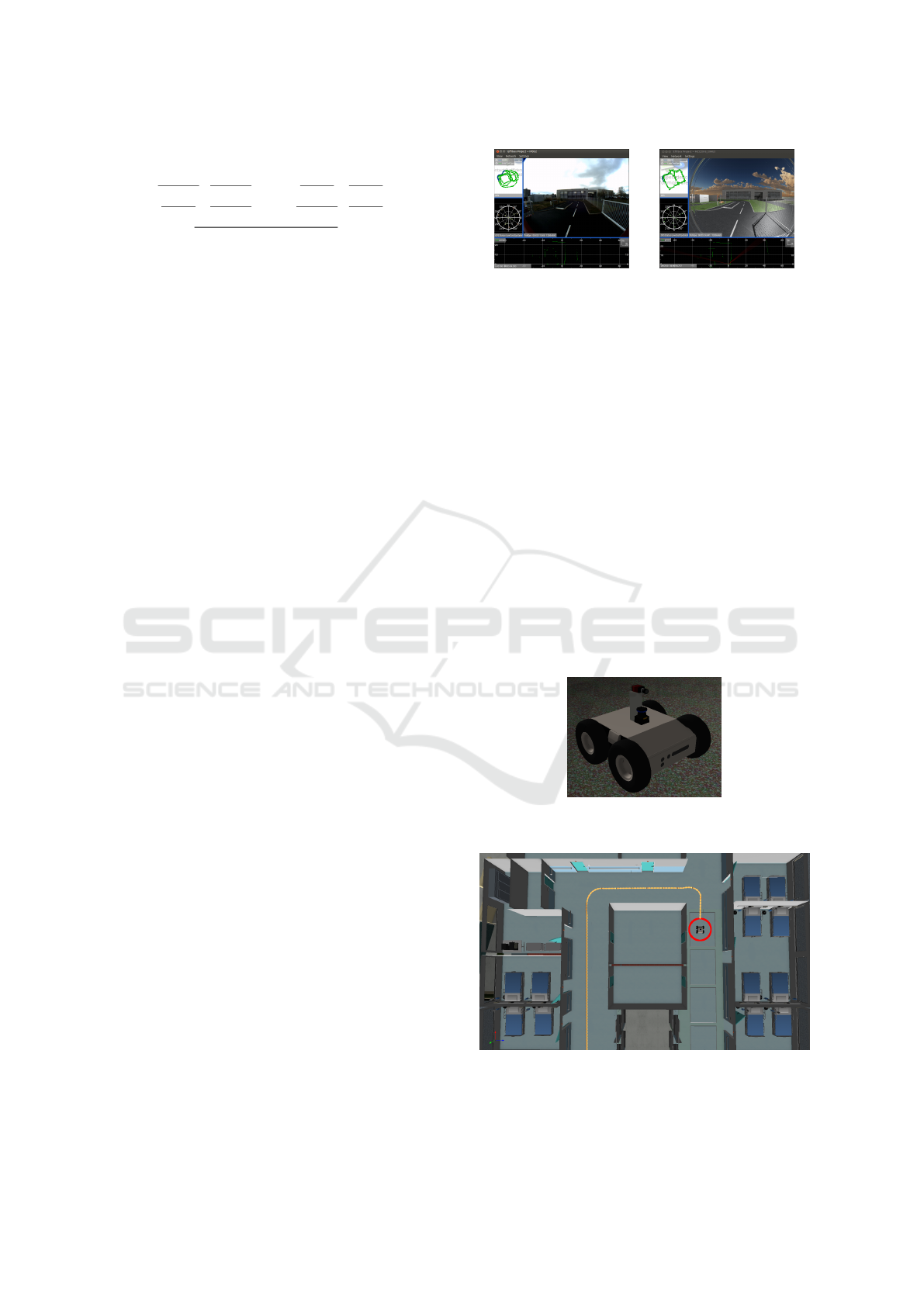
(a) Real sensors
(b) Virtual sensors
Figure 4: Comparison of Camera, GPS ans LIDAR sensors
between real data and data produced with the 4DV-Sim sim-
ulator.
which means that once the source code is validated
with the virtual platform, it can be instantaneously
carried to the real platform to be executed.
The use of a simulator also gives the opportunity
to have exact repeatability to compare the results, ac-
cess to ground truth and produce various datasets with
different environments and robot set-ups, advantages
we do not posses with experiments in real environ-
ment.
The simulated robot is a Dr. Robot Jaguar, virtu-
ally equipped with a URG-4LX Hokuyo lidar and a
640x480 global-shutter camera (pinhole model) (Fig-
ure: 5). The simulated lidar has the same parameters
than the real URG-04LX (min angle, max angle, res-
olution, frequency, etc.) and the noise added to the
measures is Gaussian distributed with parameters pro-
vided by the factory data-sheet.
Figure 5: Dr Robot Jaguar equipped with a URG-30LX li-
dar and RBG camera.
Figure 6: Simulated indoor environment containing the
robot (red circle) and command trajectory (yellow).
The environment we used is a replica of a real
ICINCO 2019 - 16th International Conference on Informatics in Control, Automation and Robotics
28
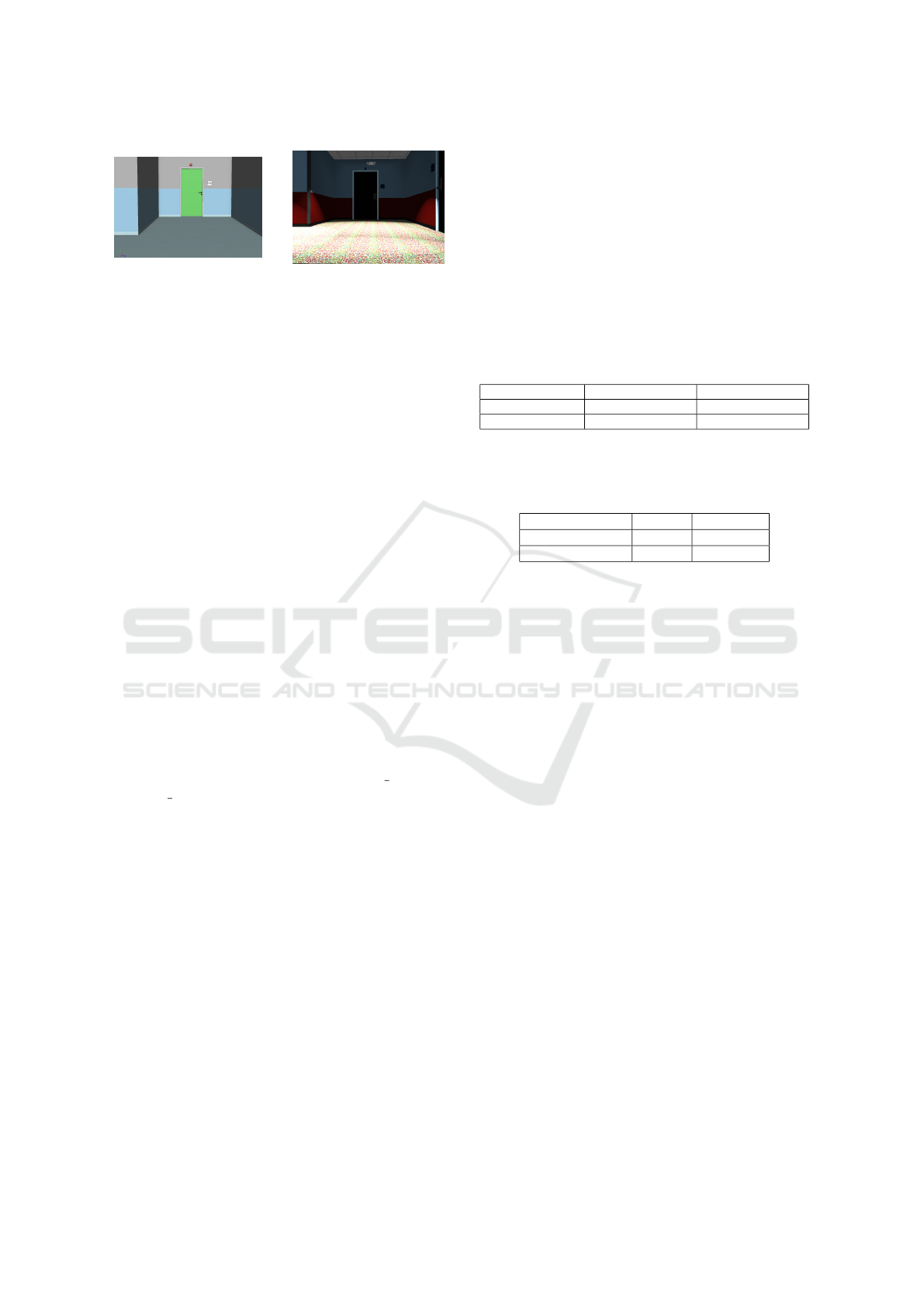
(a) Simple
(b) Complex
Figure 7: Same environment, different complexity.
American hospital (Figure: 6). All doors, doorways,
beds, hallways have the right scale and materials ef-
fects. In preliminary work, we used two different sets
of textures and lighting effects to improve gradually
the performance of the vision algorithm (Figure: 7).
4.1.1 Vision
In this section, two kinds of optimization for the Real
Time Vision step will be presented, combined, and
then discussed:
• of the algorithm: in order to detect vertical edges,
only the horizontal gradient computation is re-
quired;
• of the implementation: the data flow program-
ming model (Cabrol et al., 2005) is used, that is
to say the computation of the pixel address is re-
alized sequentially, pixel by pixel, by pointer in-
crementation.
A reference is proposed: it is a classical imple-
mentation of the Kirsh filter (Kirsch, 1971) in B&W
and color RGB imagery. In this implementation, the
computation of the pixel address is directly realized
using one multiplication and one addition. The use of
functions to access to the pixel value: get pixel()
and put pixel() increases the computing time by
30%.
For each combination (algorithm / implementa-
tion) two computing time are presented:
• the low level processing, that is to say the gradient
computation;
• the global time, where vertical segments are ob-
tained.
One can notice that the low level processing is the
most time consuming step, because the computations
are performed on each pixel of the image. Conse-
quently, the optimization of this step is the most im-
portant to realize, but it is also the most effective and
easy to realize because of the regularity of the com-
putations.
Time results are a mean using one hundred test
RGB images (in .ppm format) given by our simula-
tor on the hospital environment. As the content of the
images is roughly similar, the computing time is quite
constant. For more precision, the temporal measure-
ment is realized on a loop of one hundred iterations.
Time results are measured on a PC HP Pro-book
equipped of a processor Intel Core i5-630, at 2.4 GHz,
with 16 Go of Memory. Images are in VGA format:
640 columns × 480 lines.
In B&W imagery, the Kirsh Algorithm takes 36
ms, and the global processing leading to the detection
of the vertical segments 42,2 ms. The results for RGB
color imagery are the following, in milliseconds:
Table 1: Average computation time in milliseconds.
Algo - Impl No Opt Optimized
Kirsh: 4 Masks 111 (93 %) - 119 20 (87 %) - 22,9
Horizontal Mask 30,2 (92 %) - 32,6 10,5 (77 %) - 13,6
In term of Speed Up, the results are the following:
Table 2: Acceleration depending on the method and the op-
timization.
Algo - Impl No Opt Optimized
Kirsh: 4 Masks 1 5,19
Horizontal Mask 3,65 8,75
As a conclusion, the increase of nearly factor 9 in
computation time must be pointed out. It allows our
vertical segment detection to run at video rate (ie. in-
ferior to 40 ms) on one core. The use of less than
15 ms leaves the possibility to hook this segmenta-
tion part to other high level processing, and guaranty
a latency time of less than a video frame. Using the
SPMD programming model for the implementation of
the gradient computation and edge thinning steps, a
speed up of 3.8 is achieved using manual attribution
on the 4 cores of the RaspberryPi against 2.7 using
the Raspian load balancing.
4.1.2 Localization
We implemented the vertical detector presented pre-
viously and added the lidar data to obtain our 3D fea-
tures. In order to reduce the computation time we
limited the number of detected vertical lines and nar-
rowed this to the lines around the horizon, we can ob-
serve the projection of the 3D extracted features from
the previous image in cooperation with the lidar us-
ing camera intrinsic and extrinsic parameters (Figure:
8b).
In addition of the previous optimizations, we used
regions of interest (ROI) to reduce the number of pix-
els processed during each steps. To define these ROI,
we use the estimated position of the known feature
in the image and defined the width of the bound-
ing box using the uncertainty related to this feature
with a minimal width of 10 pixels. The height of
Camera and Lidar Cooperation for 3D Feature Extraction
29
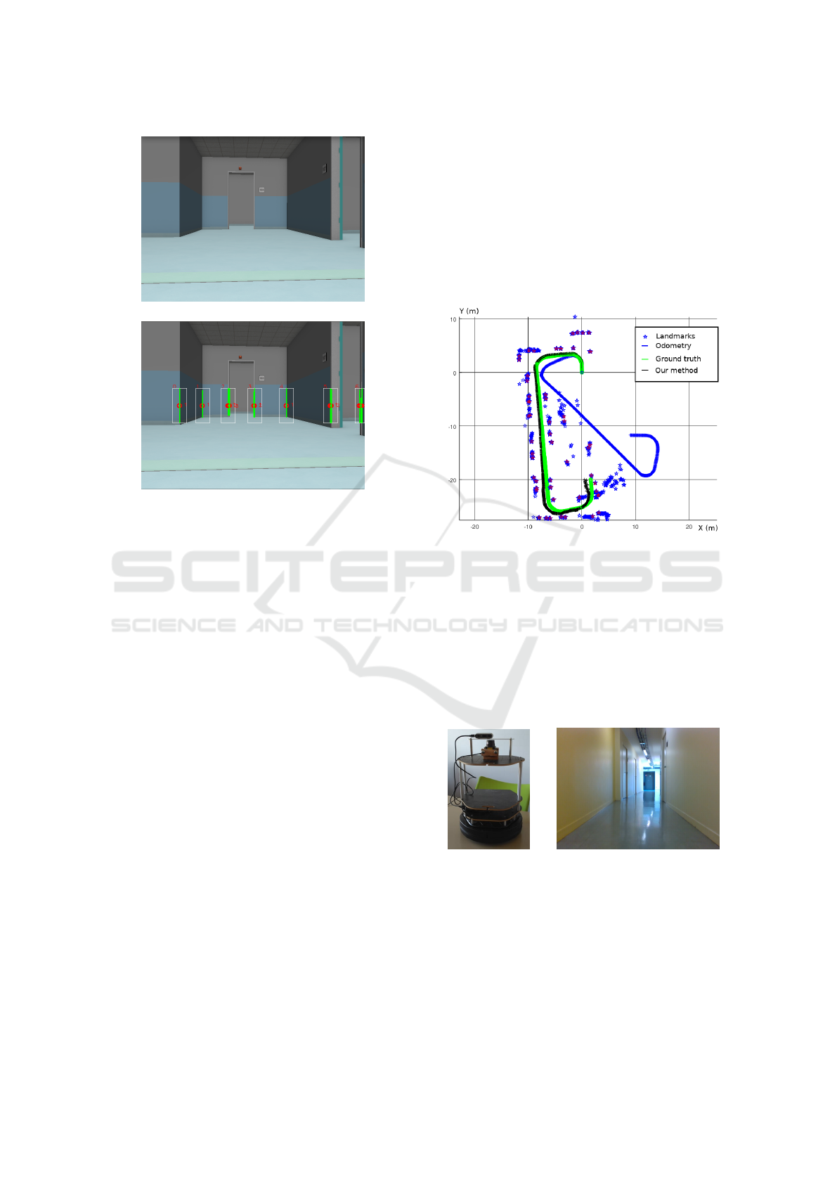
(a) Original image
(b) Features
Figure 8: Use of ROI and the 2D features results in the
SLAM map.
ROI’s bounding box is fixed to 1/4 of the image.
This is linked to the lidar’s position: every ”hit” from
the lidar will be contained within the bounding box,
whether the range is 0.5 or 30m (lidar’s minimum and
maximum range). The use of the ROI (Figure: 8b) is
extended to the full width of the image when the algo-
rithm looks for new features to add to the SLAM sys-
tem. This allows a complete scan but has to be done
at a lower frequency to save CPU-usage The average
time needed to extract verticals in a ROI is 1.6623ms.
Using a sparse SLAM system (even without multi-
threading), we can reasonably track enough features
in real time to feed a localization process.
We performed our experiment in the simulated en-
vironment using the described robot and setup; The
result is displayed in the Figure: 9. The blue stars
are the extracted and tracked features. One can rec-
ognize the shape of the building shown in top-view
from Figure: 6. The green track is the ground truth
from the simulator. The blue track is the estimated
localization using only the odometry. We can observe
the rapid drift of the odometry during turns and it’s
relative precision during forward motion. The black
track is the estimated position of the robot using the
kalman filter. The track is split in two parts, the first
part has a very precise localization (an average 2cm
error relatively to the ground truth), then a diverging
part. The second part has an increasing error is due to
a small error in heading at the moment of initialization
of new landmarks when the robot faced the hallway.
This is due to the lack of visual landmarks available
in this part of the virtual map. This slight shift added
a small angle that had repercussion on the next 25m
of evolution to a final 0.3m error over a 40m trajec-
tory. Blue stars are our observed landmarks and red
one are registered in the map created. This conclude
our virtual tests, considering that further tests should
be on a real robot to confirm the results.
Figure 9: Localization results.
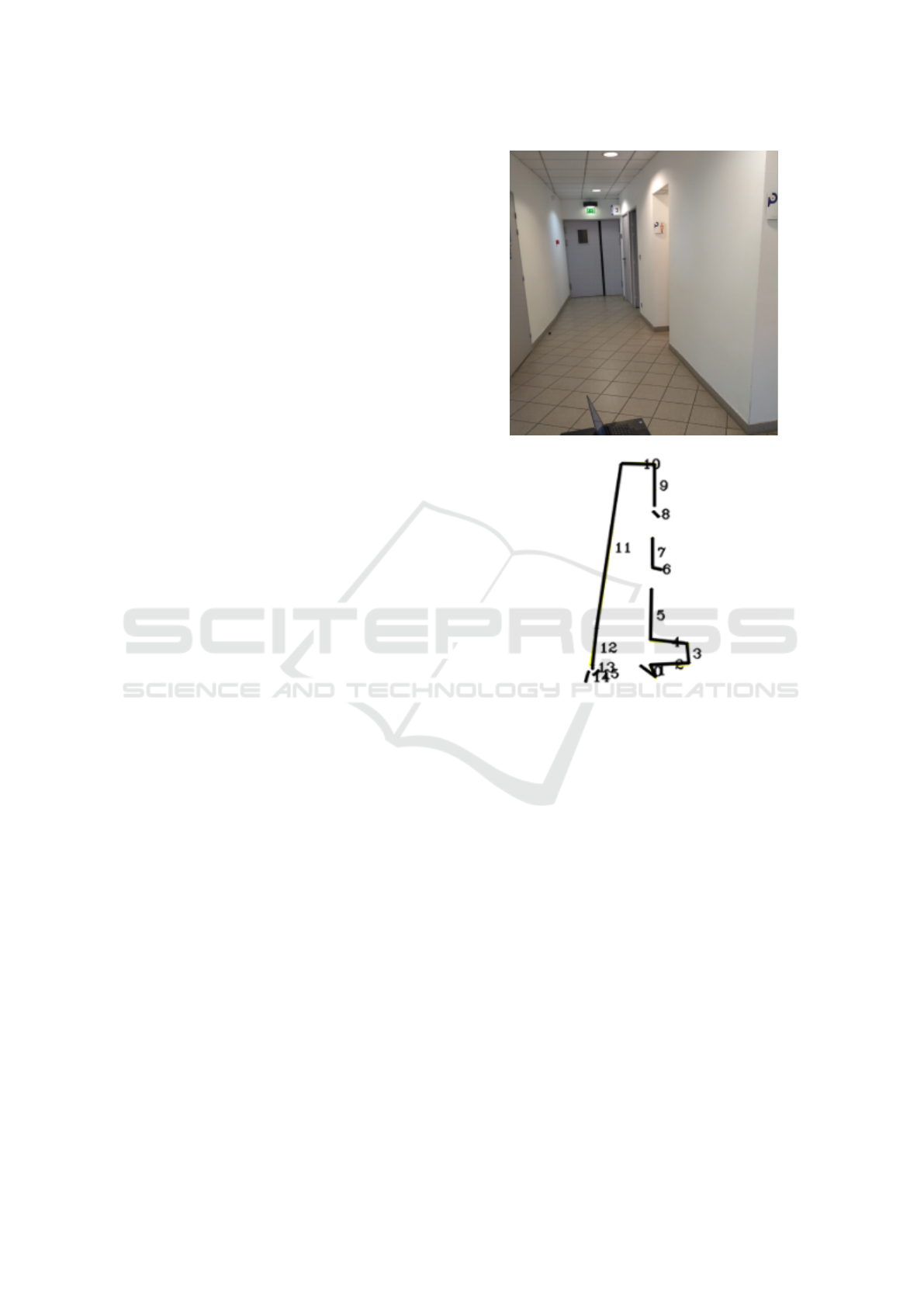
4.2 Real Experiments
Real experiment were conducted in the hallway of a
public building. We used a Kobuki TurtleBot2 plat-
form with an Hokuyo 04LX and an Intel Realsense
D435 placed on the top of the robot. The environment
we experienced in is about 40m long, having several
patio doors with large panes, solid doors and shiny
floor (Figure: 10).
(a) Real robot
(b) Hallway
Figure 10: Set-up and environment used for the experiment.
The RealSense sensor is used only to provide
a global shutter 640x480 image, we didn’t use the
RGB-D feature because it did not provide depth in-
formation with sufficient range and precision. The
corner seen on the left of the hallway is not seen at
3m (Figure: 11).
ICINCO 2019 - 16th International Conference on Informatics in Control, Automation and Robotics
30
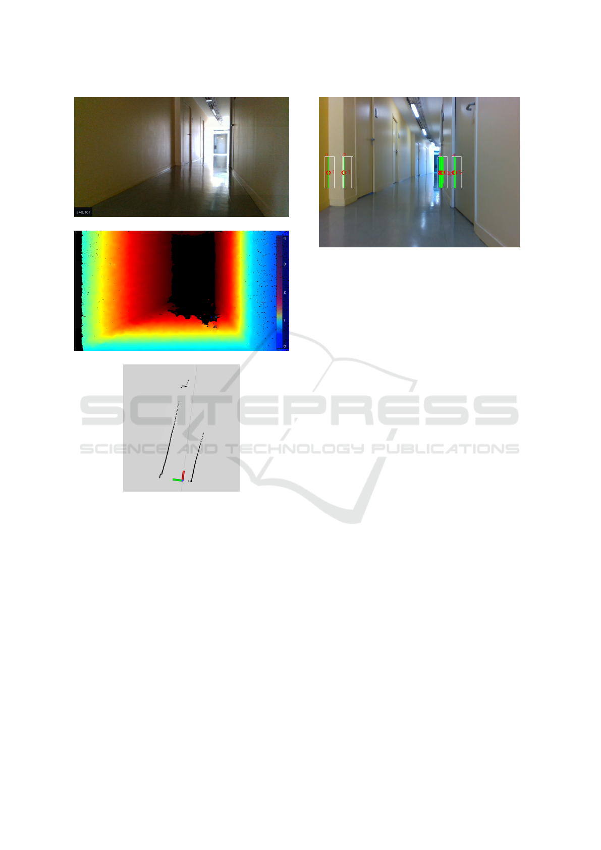
(a) Environment
(b) Intel D435
(c) Hokuyo 04-LX
Figure 11: Comparison of depth detection.
4.2.1 Localization
The real environment brought additional complex-
ity to the sensors due to two facts: the large win-
dows panes and the floor that reflects the environment.
The first issue comes from the sun light that blinds
the LIDAR sensor depending on the intensity of the
rays. The second is brought by the clean plastic floor
that create ”false” verticals in the image by reflecting
lights on the ceiling and doors. The first issue was
solved by filtering the LIDAR data while the second
one was only a matter of ROI focusing to exclude mis-
leading verticals.
Our strong initial hypothesis, 2D movement and
camera-lidar rig coplanar to the floor, is reasonable
: even with small angular errors, we still manage to
detect vertical lines in our image.
Figure 12: Detections with the real set-up.
As explained before, we do not have a proper
ground-truth available for real experiment, thus we
can’t know the exact position of the robot during the
experiment but we do have the 2D model of the build-
ing provided by the architects. This model have been
produced using precise (< 1cm) measurement by pro-
fessional surveyors, therefore, we can estimate the ef-
ficiency of the robot localization using the compari-
son between the landmarks registered by our system
and the solid shape given by exact model (black shape
in figure 13).
We compared the localization efficiency with an-
other method: the canonical scan matcher (CSM)
(Censi, 2008). We tried the ORB-Slam (Monocular)
but the complex light rendered the initialization im-
possible. Since there is no loop closing in this hall-
way, the CSM should not have particular disadvan-
tage.
On the Figure 13, we can observe the results of
the different methods. The black trajectory is the lone
odometry. The red one is the CSM result. The Blue
stars are the landmarks registered by our method, and
the trajectory is green. The odometry is outside the
building frame but not that much, contrary to the vir-
tual odometry, this one is more precise. This can be
explained by the motion method of the robot: the vir-
tual is a 4 wheeled robot and the TurtleBot is a 2
wheeled. The later present a reduced slippery dur-
ing the turns, thus reducing the error on the odometry
that made the assumption of slip-free rolling condi-
tion. The low range of the LIDAR and narrow FOV
of the camera limits the number of landmarks avail-
able but the algorithm manages to detect several of
them and successfully tracked, even with a complex
lighting.
Camera and Lidar Cooperation for 3D Feature Extraction
31
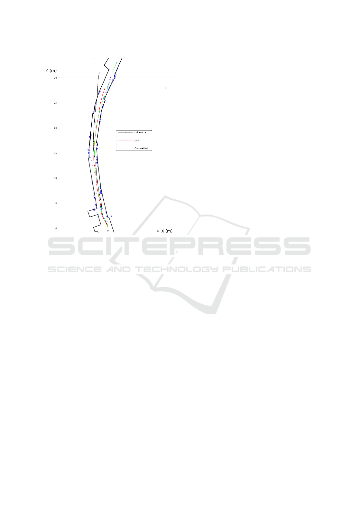
Figure 13: Localization results.
5 CONCLUSIONS
In this paper, we proposed an approach to extract fea-
tures from both camera and lidar sensors while saving
CPU-time. Upon this feature extractor, we built an
extended Kalman filter to provide fast robot localiza-
tion, re-using sensors data from others purposes. We
evaluated the interest in focused images processing to
reduce the computation time and observed a signifi-
cant improvement, enough to process all features in
real-time on a low grade computer. First, the local-
ization method has been evaluated with an advanced
robotic simulator and shown interesting results. Then
the very same algorithm was used as-is later on a real
platform, using the same sensor than the simulated
ones. The landmarks localization in the experiment
in the real hallway are conclusive regarding the 2D
model of the building. We can reasonably state that
the simulation was accurate enough to provide signifi-
cant preliminary results. It allowed a real-time testing
during the early development of the algorithm, having
incremental complexity and access to ground truth.
This helped significantly during the design of the sys-
tem before using the real robot for final and real tests.
In future work, we will focus on improvement of
the SLAM system to avoid heading shifts and include
a loop-closing method to rectify the map. The use
of RGB-D sensors to combine the image and depth
with less calibration and more accurate results is an
interesting perspective with more depth range.
ACKNOWLEDGEMENTS
This research was performed within the framework
of a CIFRE grant (ANRT) for the doctoral work of
G.Burtin at 4D-Virtualiz and LISV.
REFERENCES
Asvadi, A., Girao, P., Peixoto, P., and Nunes, U. (2016). 3d
object tracking using rgb and lidar data. In Intelligent
Transportation Systems (ITSC), 2016 IEEE 19th In-
ternational Conference on, pages 1255–1260. IEEE.
Bekris, K. E., Glick, M., and Kavraki, L. E. (2006). Evalu-
ation of algorithms for bearing-only slam. In Robotics
and Automation, 2006. ICRA 2006. Proceedings 2006
IEEE International Conference on, pages 1937–1943.
IEEE.
Burtin, G., Bonnin, P., and Malartre, F. (2018). Vision based
lidar segmentation for accelerated scan matching. In
Journal of Communications, volume 13, pages 139–
144.
Burtin, G., Malartre, F., and Chapuis, R. (2016). Reduc-
ing the implementation uncertainty using an advanced
robotic simulator.
Cabrol, A., P.Bonnin, V.Hugel, K.Boucheffra, and
P.Blazevic (2005). Temporal optimized edge segmen-
tation for mobile robotics. SPIE Optics Photonics,
Application of Digital Image Processing XXVIII, July
31st- August 4th 2005, San Diego, California, USA.
Canny, J. (1983). Finding edges and lines in images. MIT
AI Lab Tech Report TR-720.
Censi, A. (2008). An ICP variant using a point-to-line met-
ric. In Proceedings of the IEEE International Confer-
ence on Robotics and Automation (ICRA), Pasadena,
CA.
Choi, Y.-H., Lee, T.-K., and Oh, S.-Y. (2008). A line fea-
ture based slam with low grade range sensors using
geometric constraints and active exploration for mo-
bile robot. Autonomous Robots, 24(1):13–27.
De Silva, V., Roche, J., and Kondoz, A. (2018). Robust
fusion of lidar and wide-angle camera data for au-
tonomous mobile robots. Sensors, 18(8):2730.
Deriche, R. (1987). Using canny’s criteria to derive a re-
cursively implemented optimal edge detector. Inter-
national Journal of Computer Vision, 167-187.
Durrant-Whyte, H. and Bailey, T. (2006). Simultaneous lo-
calization and mapping: part i. IEEE robotics & au-
tomation magazine, 13(2):99–110.
Engel, J., Sch
¨
ops, T., and Cremers, D. (2014). Lsd-slam:
Large-scale direct monocular slam. In European Con-
ference on Computer Vision, pages 834–849. Springer.
ICINCO 2019 - 16th International Conference on Informatics in Control, Automation and Robotics
32

Engelhard, N., Endres, F., Hess, J., Sturm, J., and Burgard,
W. (2011). Real-time 3d visual slam with a hand-held
rgb-d camera. In Proc. of the RGB-D Workshop on
3D Perception in Robotics at the European Robotics
Forum, Vasteras, Sweden, volume 180, pages 1–15.
Huang, H. (2008). Bearing-only SLAM : a vision-based
navigation system for autonomous robots. PhD thesis,
Queensland University of Technology.
Kalman, R. E. (1960). A new approach to linear filtering
and prediction problems. Transactions of the ASME–
Journal of Basic Engineering, 82(Series D):35–45.
Kirsch, R. (1971). Computer determination of the con-
stituent structure of bio1ogical images. Computers
and Biomedical Research 4, 315-328.
Lemaire, T. and Lacroix, S. (2007). Monocular-vision based
slam using line segments. In Robotics and Automa-
tion, 2007 IEEE International Conference on, pages
2791–2796. IEEE.
Micusik, B. and Wildenauer, H. (2015). Descriptor free vi-
sual indoor localization with line segments. In Pro-
ceedings of the IEEE Conference on Computer Vision
and Pattern Recognition, pages 3165–3173.
Mur-Artal, R., Montiel, J. M. M., and Tardos, J. D. (2015).
Orb-slam: a versatile and accurate monocular slam
system. IEEE Transactions on Robotics, 31(5):1147–
1163.
Nachar, R., Inaty, E., Bonnin, P., and Alayli, Y. (2014).
Polygonal approximation of an object contour by de-
tecting edge dominant corners using iterative corner
suppression. VISAPP International Conference on
Computer Vision Theory and Applications, pp 247-
256, Jan 2014, Lisbon, Portugal.
Newcombe, R. A., Lovegrove, S. J., and Davison, A. J.
(2011). Dtam: Dense tracking and mapping in real-
time. In Computer Vision (ICCV), 2011 IEEE Inter-
national Conference on, pages 2320–2327. IEEE.
Premebida, C., Monteiro, G., Nunes, U., and Peixoto, P.
(2007). A lidar and vision-based approach for pedes-
trian and vehicle detection and tracking. rn, 10:2.
Prewitt, J. (1970). Object enhacement and extraction. Pic-
ture processing and Psychopictorics, BS. Lipking and
A.Rosenfield ed, Academic Press.
Pumarola, A., Vakhitov, A., Agudo, A., Sanfeliu, A.,
and Moreno-Noguer, F. (2017). Pl-slam: Real-time
monocular visual slam with points and lines. In
Robotics and Automation (ICRA), 2017 IEEE Inter-
national Conference on, pages 4503–4508. IEEE.
Roberts, L. (1965). Machine perception of 3d solids. Opti-
cal & electro optical information processing, JP.Tipett
and al., Cambridge, MIT Press.
Roumeliotis, S. I. and Bekey, G. A. (2000). Segments: A
layered, dual-kalman filter algorithm for indoor fea-
ture extraction. In Intelligent Robots and Systems,
2000.(IROS 2000). Proceedings. 2000 IEEE/RSJ In-
ternational Conference on, volume 1, pages 454–461.
IEEE.
Schramm, S., Rangel, J., and Kroll, A. (2018). Data fusion
for 3d thermal imaging using depth and stereo camera
for robust self-localization. In Sensors Applications
Symposium (SAS), 2018 IEEE, pages 1–6. IEEE.
Sobel, I. (1978). Neighborhood coding of binary images for
fast contour following and general binary array pro-
cessing. Computer Graphics and Image Processing
vol 8,.
Von Gioi, R. G., Jakubowicz, J., Morel, J.-M., and Randall,
G. (2012). Lsd: a line segment detector. Image Pro-
cessing On Line, 2:35–55.
Zuo, X., Xie, X., Liu, Y., and Huang, G. (2017). Robust vi-
sual slam with point and line features. arXiv preprint
arXiv:1711.08654.
Camera and Lidar Cooperation for 3D Feature Extraction
33
