Simulation of Racing Greyhound Kinematics

Md Imam Hossain

, David Eager

and Paul Walker

Faculty of Engineering and Information Technology, University of Technology Sydney, Sydney,

PO Box 123, Broadway 2007, Australia

Keywords: Greyhound Racing, Greyhound Kinematics, Dynamic Simulation, Numerical Simulation, Rigid Body

Dynamics, Injury Prevention, Animal Welfare.

Abstract: This paper outlines greyhound dynamics results for yaw rate, speed, and the congestion pattern during a race

derived through numerical modelling. The simulation results presented are also correlated to actual race data

to validate modelling performance and reliability. The tasks carried out include the development of a

numerical model for greyhound veering and race related supporting models, creating track 3D models

replicated from actual survey data of the track, establishing a simulation environment that emulates an actual

greyhound race, and the processing of both simulation and actual race data. The results show that greyhounds

are susceptible to experience varying high acceleration in first five seconds into the race, during which a

minimum average forward acceleration of 3.9 m/s

was calculated, a peak yaw rate magnitude of 0.4 rad/s

before the bend while transitioning into the track, and congestion during a race is affected by lure driving

performance.

1 INTRODUCTION

Greyhound racing is a popular sport in many

countries where the industry is thriving. Gradually,

focus is changing to best-racing performance

outcomes while minimising race injuries on the

tracks. As a result, simulation of greyhound racing

becoming an increasingly important technique for

evaluating races as it would directly and indirectly

benefit many parties including track designers, race

operations managers to name few.

When it comes to the greyhound, they are able to

travel by a maximum speed averaging above 70 km/h

on the land. This astonishing speed is achieved

through galloping gait of a greyhound which is also

preferred gait for most quadrupedal mammals

(Krasny, and Orin, 2004). However, musculoskeletal

injuries are a common happening in racing

quadrupeds such as greyhounds when compared to

non-racing quadrupeds (Sicard et al., 1999). A study

showed that various track dynamic conditions, as well

as greyhound running speed, have a significant

influence on race performance and injuries (Iddon et

https://orcid.org/0000-0002-1246-3454

https://orcid.org/0000-0003-1926-7867

https://orcid.org/0000-0003-3988-3966

al., 2014, Mahadavi et al., 2018, Hasti et al., 2017a).

Likewise, investigation of five tracks showed that

factors such as track surface grades, achievable speed,

and race distance resulted significant effect on

greyhound injury rates (Iddon et al., 2014). Moreover,

various observations of racing greyhound injuries

indicated that congestion at the start of the race as

well as at the immediate bend in the track is a

precursor to major race injuries (Hayati et al., 2017b).

For greyhound racing, a traditional approach for

analysing race dynamics can be cumbersome and

difficult to achieve. This is because traditional

techniques such as graphical and analytical methods

sometimes lack accuracy and the complexity can

increase exponentially for a relatively simple

practical problem (Garcia et al., 2012). An alternative

solution is numerical analysis and methods through

fast processing of alphanumeric data, data

formulation and computational methods (Garcia et

al., 2012). In the numerical approach, mathematical

models are developed from observation of physical

and technical processes where derived equations are

computed at discrete points in the time (Griebel et al.,

2010). Furthermore, the availability of corresponding

Hossain, M., Eager, D. and Walker, P.

Simulation of Racing Greyhound Kinematics.

DOI: 10.5220/0007829000470056

In Proceedings of the 9th International Conference on Simulation and Modeling Methodologies, Technologies and Applications (SIMULTECH 2019), pages 47-56

ISBN: 978-989-758-381-0

physical or technical processes results would allow

verification of numerical results or improvements to

developed numerical model methods (Griebel et al.,

2010).

This paper describes the design and mechanism of

dynamic numerical models for conducting greyhound

racing simulation which is processing efficient and

yet robust enough to extract various greyhound

kinematics and racing dynamics, which include

greyhound yaw rate, speed, congestion pattern,

greyhound path following as well as factors which

affect racing performance. Furthermore, the design

and mechanism described can be expanded and

utilised in other prospective areas such as vehicle and

quadruped running simulations with multiple

interacting factors having proper constraints in place.

The realistic constraints are such that any dynamic

system models developed exhibit controllability of

the numerical algorithms output convergence

(Respondek, 2010). This is because controllability of

dynamical systems allows extension of dynamic

systems conditions for given problems (Respondek,

2005).

Moreover, this paper analyses simulation and

actual race data for deriving trends in racing

greyhounds. The simulation carried out were matched

to available field data configuration such as eight

greyhounds running over a defined distance in a track

which has two bends track paths as well as two

straights track paths.

2 MATHEMATICAL MODEL

DEVELOPMENT OVERVIEW

To create a viable model for greyhound racing, there

are various variables which first need to be identified

and addressed. These variables may come from

within the racing track or from the greyhound. By

considering racing track and greyhound as different

systems their inherent system behaviour defining

variables can be identified. Furthermore, race

operational configuration and running conditions

define a system which by emulating it creates

necessary inputs for a simulation model of greyhound

racing.

2.1 Model Scope

When a greyhound is racing, its motion can be

defined and traced in term of displacement, velocity,

and acceleration in Euclidean space. While the

nominal acceleration of greyhound can be directly

related to forces acting on it, deriving of the

instantaneous displacement and velocity of

greyhound can be a complex task. This is because the

instantaneous displacement and velocity of a

greyhound in racing not only depend on the racing

track design and racing operational running

conditions but also rely on the adjacent greyhounds’

dynamic profiles. This creates a greater

unpredictability in the controllability of a

greyhound’s instantaneous displacement and velocity

during a race. Furthermore, observation has

confirmed that a racing greyhound can bump into

another adjacent greyhound as well as follow a

particular path, which is not defined by its motion

limiting force factors but are an inherent part of race

dynamics. Consequently, the interactions between

greyhounds in a race have a significant impact on the

greyhound race dynamics. A greyhound veering

model is developed which outputs greyhound

locations during a race from the start of the race till

the end. The model predicts the path taken by

individual greyhounds during a race while having

each greyhound its own character in terms of

velocities. Finally, the model calculates adjacent

greyhounds’ locational, track design and race

operational influences and optimises potential

locations of greyhound during a race. In the simplest

form, the model can be described by a finite

dimensional system state equation. This model is said

to be controllable if and only if the control variable

would allow the system to reach any final state in the

control space in the finite time from any given initial

state (Respondek, 2005).

2.2 Understanding of Greyhound

Racing Elements

There are a number of distinct elements which take

part in a greyhound racing. While some of these

racing elements are dynamic in nature, there are also

elements which are static and have a great impact on

a racing greyhound. The main dynamic bodies in

racing are the lure during a race, adjacent racing

greyhounds, and individual greyhound limbs which

are required for greyhound locomotion. The

fundamental static bodies relating to racing are race

starting boxes locations and orientations relative to

track, track surface properties including surface

traction, impact attenuation qualities, track camber,

and track racing line. During a race, lure, starting

boxes, and track are regulated to certain degrees that

their behaviours are controlled and follow a specific

predefined pattern.

SIMULTECH 2019 - 9th International Conference on Simulation and Modeling Methodologies, Technologies and Applications

2.3 Model Composition and

Mechanism

By considering a greyhound as a point object its

overall motion in a race can be formulated by

knowing the factors which induce the motion as well

as the factors which alter the motion characteristics as

a result of combined racing environmental and

greyhound limits. The main driving factor for

greyhound motion is greyhound stride while the

motion altering factors are greyhound natural steering

limits, collision in a race, track geometry and surface

condition, lure velocity profile and track boundaries.

These discrete factors are modelled using kinematics

and vectors equations where kinetics equations and

input to output unit tests are used for finding initial

and final values for the model equations.

Superposition principle is applied to the model

equations to solve for aggregated results of discrete

race dynamics factors and calculate greyhound

location during a race using Euler's method. The

summation of discreet factors can be expressed as

V(v

+ v

)

= V(v

) + V(v

) +

V(v

) + V(v

)

(1)

In which V is the final velocity vector function for

... v

discrete factors of race dynamics. The v

factor represents greyhound stride acceleration

velocity due to the sum of all the forces exerted by a

greyhound’s stride which can be modelled using

Newton’s second law (2). This is also the forward

acceleration of greyhound. It was assumed that a

greyhound’s exerted stride force remains constant for

the entire race duration although, in reality, data show

greyhound acceleration is highly variable during the

first three strides. However, as the time fraction of the

first three strides is relatively small compared to

entire race duration, a linear acceleration model and

an averaged value of greyhound maximum

accelerations are appropriate for getting stable final

velocity output. For constant acceleration, greyhound

maximum forward acceleration is calculated using

Eq. 3 where greyhound final velocity (v) is 19.4 m/s,

greyhound displacement (s) for reaching final

velocity is 15 m and initial velocity (v

) is 0 m/s. This

maximum forward acceleration is plugged into Eq. 4

to calculate the greyhound stride acceleration velocity

factor v

. In Eq. 4, v

is greyhound velocity in

previous time instant and dt is the time elapsed

between v and v

∑ F = ma

(2)

v2 = v

+ 2 * a

* s

(3)

v = v

+ a

* dt

(4)

The purpose of the v

factor is to provide

greyhound the motivation to race as well as steer

greyhound heading as it moves in the track.

Therefore, this factor is a function of greyhound’s

lure line of sight, frictional force, and centrifugal

force vectors. However, observation of greyhound

race and race data have confirmed that lure line of

sight is a significant guiding influence for greyhound

path following around the track in absence of other

influences such as congestions due to adjacent racing

greyhounds. As a result, the lure line of sight vector

was considered also a function of frictional force, and

centrifugal force vectors (Eq. 5). The lure line of sight

vector is constructed from lure and greyhound

instantaneous locations in the track. The frictional

force has two components where one is due to track

camber (θ) and another one is the nominal friction due

to greyhound instantaneous velocity as denoted by m

* g * sin θ and C * v respectively.

Lure line of sight vector = lure line of sight

vector + centrifugal force vector + paw and

track surface frictional force vector

(5)

Centrifugal force = m * v

/ R

(6)

Greyhound paw and track surface frictional

force = (m * g * sin θ) + (C * v)

(7)

In Eq. 6, R is instantaneous radius of curvature of

greyhound path following and m is greyhound mass.

In Eq. 7, m is greyhound mass and C is a constant.

The v

factor is a tweaking vector to v

factor to

achieve precise greyhound heading movement

without which results in unnatural greyhound heading

movement behaviour. The reason for this, in real-

world greyhound heading direction change does not

go through step change to meet the lure following

path instead it goes through many mini-movements to

catch up lure following path. This creates a lag

between greyhound spotting lure location and

greyhound merging with the lure following path.

Moreover, greyhound has physical turning limits at

an instant. All of these phenomena are modelled using

a steering vector which is a function of greyhound

current heading direction vector and lure line of sight

vector.

Steering vector = lure line of sight vector –

current heading direction vector

(8)

Simulation of Racing Greyhound Kinematics

The v

final velocity factor determines the

outcome of greyhound checking and bumping as well

as greyhound collision avoidance tendency to

adjacent greyhound during a race which results in

greyhound surrounding aware variable velocities.

These situations in a race are modelled by using a

collision avoidance vector which successively finds

greyhounds in proximity and through a number of

iterations construct a clearance vector. The exact

number of iterations was chosen based on simulation

time stamps and convergence of the clearance vector.

Furthermore, by assuming there is no collision

between two greyhounds vertically, circle to circle

collision detection is used for checking overlapping

greyhounds.

Collision avoidance vector = location vector of

greyhound in proximity – location vector of

greyhound

(9)

Clearance vector = current heading direction

vector – collision avoidance vector

(10)

The v

factor finds the effect of track cross falls

on greyhound veering. As the effect of cross fall can

be proportional to track banking angle (θ) at spot

location, a linear calibrated force is used along with

normal force vector for calculation. To find banking

angle at a given location in track, the track surface is

discretised using small triangles where the vertices of

each triangle are used for finding normal force vector

(N) and corresponding bangle angle (θ).

= U

* V

– U

* V

(11)

= U

* V

– U

* V

(12)

= U

* V

– U

* V

(13)

Normal force vector (N) magnitude =

m * g * cos θ + (C * v)

(14)

Where, U = p

- p

and V = p

– p

for p

, p

triangle vertices and m is greyhound mass and C is a

constant.

While racing greyhound avoids colliding with

track boundaries like inside lure rail. The v

factor is

used for applying a track boundary collision

avoidance vector to final velocity vector. For this

purpose, track boundaries are sampled with a number

of evenly spaced points and by using nearest points to

greyhound location boundary collision avoidance

vector is found.

Boundary collision avoidance vector =

location vectors of adjacent points on track

boundaries – location vector of greyhound

(15)

The v

factor models variable track surface

conditions at different track locations as well as

variable greyhound stride acceleration from greyhound

to greyhound for the race period. Modelling of variable

track surface conditions is essential, as, despite

identical stride from a greyhound over the race period,

non-uniform track surface conditions such as hardness,

softness, and coefficient of friction determine

greyhound stride acceleration. This factor is a function

of stride duration, race time, and a random number

generator.

The v

factor adds a specific greyhound behaviour

to final velocity vector which occurs when a greyhound

is lagging behind the lure significantly as observed

from various races. It was noticeable that greyhound

maintains an additional offset distance from track

inside boundary to get a better sight of the lure

depending on the distance between greyhound and

lure. However, various races also indicate that this

specific behaviour varies from greyhound to

greyhound. This situation is modelled by constructing

a boundary offset vector which is a function of

greyhound distance to lure, minimum offset from the

boundary and a constant as given below:

Boundary offset vector = minimum offset

from boundary * (distance to lure / C)

(16)

Where minimum offset from boundary and C are

calibrated to be 0.5 m and 5 m respectively.

The v

factor defines lure motion in terms of track

path and leading greyhound location in the race. For

this factor, a model function is created which takes into

account of track predefined lure travel path and lure

and leading greyhound separation distance to provide

lure instantaneous velocity which would maintain lure

driving for the duration of a race while maintaining a

separation distance. The model function first calculates

heading direction of the lure by copying track

curvature profile and then set lure instantaneous speed

based on the lure and leading greyhound separation

distance. The setting of lure instantaneous speed (S) is

based on the following rules where the constants were

tweaked to meet the lure driving performance:

((A > B → (C > 30 → X = 1.9489)) ∧ (A > B

→ (C > 20 → X = 3.3378)) ∧ (A > B → (C >

15 → X = 6.1156)) ∧ (A > B → (C > 10 → X

= 8.893)) ∧ (A > B → (C > 5 → X =

16.9489)) ∧ (A > B → (C > 1 → X = 17.504))

∧ (A > B → (C > 0.2 → X = 17.782))) ∧ ((A

14 → X = 14)) ∧ (A

10 → X = 18.62)) ∧ (A 5 → X =

17.504)) ∧ (A 1 → X = 16.9489))

∧ (A 0.2 → X = 20))

(17)

SIMULTECH 2019 - 9th International Conference on Simulation and Modeling Methodologies, Technologies and Applications

In which A is distance between leading greyhound

and lure, B is maintaining separation distance, C is

the difference between A and B, and finally X is lure

instantaneous speed.

Finally, in the greyhound motion model

composition, vertical acceleration velocity factor was

neglected since instantaneous vertical velocity is

negligible compared to other greyhound velocity

influencing factors because of low track surface

penetration by greyhound paw during galloping in a

race.

3 SIMULATION PLATFORM

The Blender software package was used as the

simulation platform for creating contents for

simulation visualisation as well as implementation,

setup and data extraction of the simulation models

using Python programming language. First, race track

3D model was imported into Blender virtual

Euclidean space from track survey data where it is

constructed and formatted to meet the needs of

mathematical models. Then, racing elements 3D

models such as starting boxes, greyhounds, lure and

shape defining objects such as track boundary curves

were created in Blender virtual Euclidean space

meeting mathematical model requirements. Finally,

the Blender Python application programming

interface was used for writing simulation code inside

Blender software package. The primary components

of simulation code are: greyhound object which

defines a greyhound’s dynamic model as well as it’s

state in a particular time stamp, a lure object which

defines lure dynamic model and its state in a

particular time stamp, a method for calculating

collision between greyhounds, and a method

containing code for simulation numerical solver and

updating 3D models in Blender virtual Euclidean

space. For both lure and greyhounds’ motions, the

numerical solver calculates time-varying behaviour

of each dynamic system by solving models functions

and numerical integration using Euler method where

the results from each model function are compounded

using superposition principle. For example, the final

location of each dynamic object is determined by

integrating the velocity over time as follows:

S = ∫v * dt

(18)

new

= S

old

+ v * dt

(19)

Where S

new

is the new location, S

old

is the old

location, v is instantaneous velocity and dt is the

smallest unit of time in simulation.

The global variables in the simulation setup are

lure initial speed, lure maintaining acceleration, lure

starting acceleration, greyhound maximum average

acceleration, greyhound maximum speed, greyhound

minimum speed, lure greyhound separation distance,

starting boxes locations and orientations, and lure

offset from the starting boxes before racing. These

variables were adjusted to match greyhound races.

4 SIMULATION RESULTS AND

PERFORMANCE EVALUATION

To validate greyhound racing model simulation

results greyhound race data were retrieved from

IsoLynx system. The IsoLynx system captures real-

time greyhound coordinates data during a race where

it can trace a greyhound’s location in the track in

terms of X and Y coordinates relative signal towers.

Different races greyhound coordinate data from both

simulation results and actual race were used for

validating simulation models performances. The

races which were selected from both simulation and

actual race have identical setups in terms racing time

of the day, racing distance to rule out unknown

factors affecting the comparisons as well as to find

different racing factors general trends. Moreover,

simulation and race data were resampled to match

greyhound stride duration since greyhound dynamics

state is reflected with every stride. Finally,

simulations were run with slightly varying lure

driving, greyhound maximum acceleration behaviour

configurations from nominal values to exaggerate the

effects of different racing factors outcomes. The

following sections analyses model simulation

performance to race data.

4.1 Greyhound Performance Indicators

The following major greyhound kinematics variables

were analysed.

4.1.1 Path Following

As greyhound races, they follow a specific path in the

track. The following graphs show X and Y

coordinates of a single greyhound during a race. The

graphs show that greyhound path coordinates shape

from simulation model results closely match with

race data. By looking into rate change of coordinates

subtle differences were also analysed. The maximum

and minimum percentage differences between

simulation and race for X coordinates are 6% and 7%

respectively. The maximum and minimum

Simulation of Racing Greyhound Kinematics

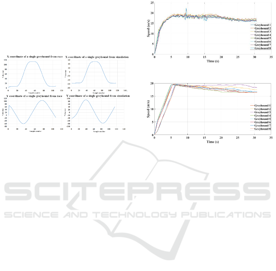
percentage differences between simulation and race

for Y coordinates are 4% and 15% respectively. This

shows simulated models resulted in a highly accurate

path following while percentages differences can be

attributed to slightly different race configurations

between simulation and actual race and varying

nature of each race.

Figure 1: Greyhound coordinate data as produced from

simulation and race.

4.1.2 Speed and Acceleration

During a race a greyhound’s speed remains variable

and has different phases as found from simulation and

race data. The following graphs depict greyhound’s

instantaneous speeds versus time for both simulated

and actual races. As shown in Figures 2 and 3, the

greyhound has an initial high acceleration phase

which puts a greyhound into its maximum speed limit

of roughly 19.5 m/s where the overall duration of this

phase depends on race distance, track shape and

starting box location in the track. Both simulated and

actual race data show initial acceleration continues

for 5 s where the rate change of this initial

acceleration is highly variable for actual race whereas

for simulation it is fixed as the greyhound model

functions use a constant average maximum

acceleration for greyhounds. After an initial

acceleration phase reaching maximum speed

greyhounds tend to lose speed as the time passes as

shown in the Figures 2 and 3. The average

deceleration of greyhound in this phase is

approximately 0.13 m/s

as found from both

simulation and race. Finally, the local fluctuations in

greyhounds speed can be attributed to factors

including track surface effects, bumping and

checking of greyhounds, and specific individual

greyhound behaviour.

Figure 2: Greyhound speed during a race.

Figure 3: Greyhound speed during a race from simulation.

4.1.3 Yaw Rate

Yaw rate is an important aspect in greyhound

kinematics as it defines how quickly a greyhound is

turning its heading. Also, veering performance during

a race as well as the lateral force magnitude acting on

a greyhound can be traced from the yaw rates.

Figures 4 and 5 illustrate instantaneous yaw rate of a

greyhound as derived from simulated and actual races

data. For the race distance selected, there are two bends

of constant radius in the track which are visible in the

yaw rates Figure 4 (red regions) where a yaw rate of

approximately 0.37 rad/s means the greyhound is

having a turning of radius roughly 50.5 m while

traversing through the bends with a speed roughly 18.8

m/s. Also, it is noticeable there is an initial spike in the

yaw rate of about 0.4 rad/s at 2.84 s and 1.49 s for

simulation and race data respectively. This is because

race distance start box location is not perfectly aligned

with the track path which causes the greyhound to

make an initial sharp turn for transitioning into the

track. The local fluctuations in the yaw rates can be

caused by greyhound path deviation because of

bumping and checking or collision avoiding. Overall,

the simulated race shows an excellent agreement with

the actual race data.

SIMULTECH 2019 - 9th International Conference on Simulation and Modeling Methodologies, Technologies and Applications

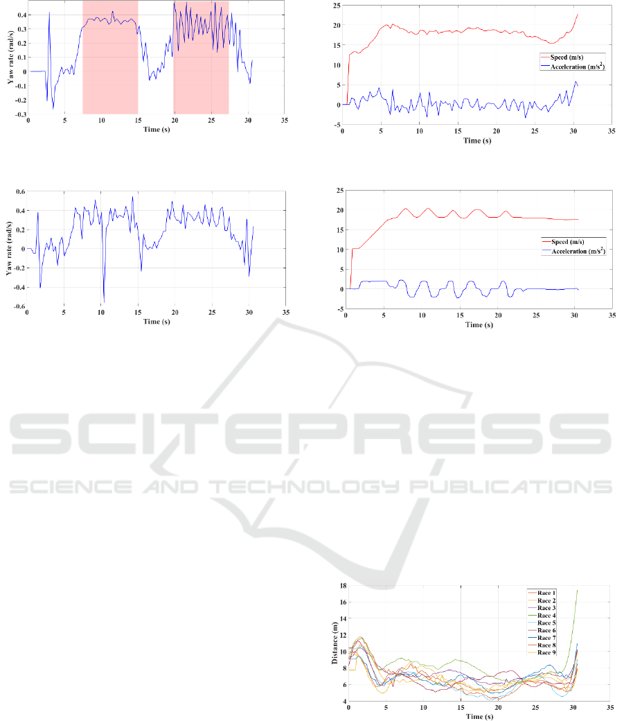
Figure 4: A greyhound’s yaw rate during a race from

simulation.

Figure 5: A greyhound’s yaw rate during a race.

4.2 Lure Performance Indicators

The following major lure performance variables were

analysed.

4.2.1 Speed

Lure driving condition was analysed between

simulation lure model and the actual race. The

simulation model yielded better lure driving

performance than the actual race as shown in Figures 6

and 7. The overall rate change of lure speed is higher

in the actual race and lower in the simulation model.

Furthermore, in actual race lure speed was affected by

track shape such as around the bends the overall speed

was slightly lower whereas no such trends are

noticeable in the simulation model other than

fluctuations from overall speed.

Finally, it is expected that both simulation model and

actual race lure driving would be slightly different

from each other as every race is unique in terms of

greyhound kinematics which lure highly depended on.

Figure 6: Lure driving speed during a race.

Figure 7: Lure driving speed during a race from simulation.

4.2.2 Lure Separation Distance

Maintaining a safe distance from the leading

greyhound in the race is also a performance indicator

for lure driving condition. The following figures

shows the simulation model and actual race lure

separation distance from leading greyhound during

races. As can be seen, in the actual race lure

separation distance tend to become lower and lower

until 20 s into the race where it was increased and

lowered again. In the simulation model, lure

separation distance is steadier after initial phase and

was increased after approximately 21 s into the race.

Figure 8: Lure separation distance from different races.

Simulation of Racing Greyhound Kinematics

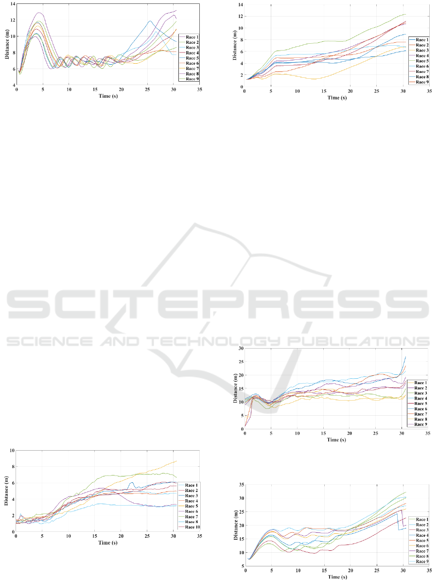
Figure 9: Lure separation distance from different simulated

races.

4.3 Greyhound Racing Performance

Indicators

To measure the racing performance the following

major variables were analysed.

4.3.1 Mean Distance from Cluster Centroid

In the race, greyhounds pack can be considered as a

cluster where the distances of each individual

greyhound from the cluster centroid can be averaged

to calculate the mean distance from cluster centroid.

Mean distance from cluster centroid can be used as a

measure to identify greyhounds pack formation and

resulting pack density. Figures 10 and 11 show

differences between simulated and actual race mean

distance from cluster centroid. Evidently, in actual

race greyhounds pack remained tightly packed as

indicated by the low mean distance from cluster

centroid value of about 2 m until 7 s into the race and

then mean distance saw a gradual increase until the

end of the race. In simulation, greyhounds pack

density was reduced more rapidly in the first 5 s into

the race and then it saw a slow and gradual increase

until the end of the race. Overall, both simulation and

actual race showed a similar trend in the greyhound

pack density.

Figure 10: Greyhounds mean distance from cluster centroid

for different races.

Figure 11: Greyhounds mean distance from cluster centroid

for different simulated races.

4.3.2 Mean Distance from Lure

Like lure separation distance, the mean distance from

lure is the average of all individual greyhound

distances from the lure during a race. A higher value

of the mean distance from lure indicates greyhounds

more spread out along the track while going through

different packs formations. As can be seen from the

Figure 12, in actual race mean distance from lure

slowly increases after initial greyhound acceleration

phase. In the simulation, after the initial acceleration

phase, the mean distance from lure remains mostly

steady until approximately 15 s into the race while

after this period it increases significantly. As a result,

both simulation and actual race show that mean

distance from lure increases with time during a race

which indicates that dispersing of greyhounds is

proportional to race time.

Figure 12: Greyhounds mean distance from lure for

different races.

Figure 13: Greyhounds mean distance from lure

for different simulated races.

SIMULTECH 2019 - 9th International Conference on Simulation and Modeling Methodologies, Technologies and Applications

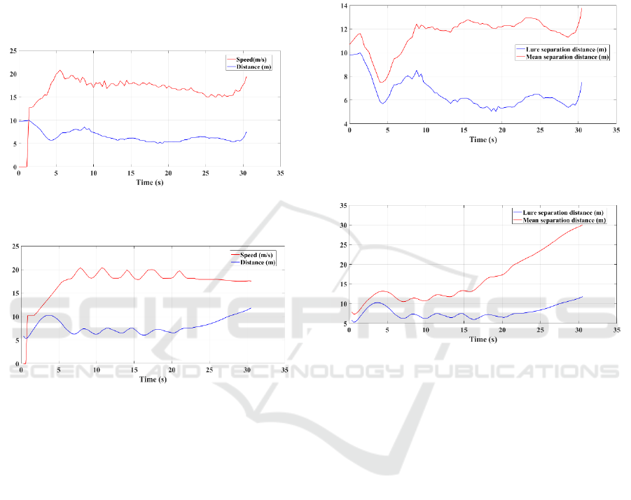
4.3.3 Speed vs. Separation Distance

Both simulation and actual race data showed that

there is an approximate inversely proportional

relationship between lure speed and lure separation

distance which is shown in Figures 14 and 15. The

instantaneous increase in lure speed decreases the lure

separation distance and vice versa. This observed race

dynamic nature can be utilised to design race dynamic

nature outcomes.

Figure 14: Lure speed vs. lure separation

distance during a race.

Figure 15: Lure speed vs. lure separation distance

during a race from simulation.

4.3.4 Lure Speed vs. Mean Distance from

Cluster Centroid

Both simulation and real race data indicated no

influence of instantaneous lure speed on mean

distance from cluster centroid dynamic results.

4.3.5 Lure Speed vs. Mean Distance from

Lure

Both simulation and real race data did not show any

direct relationship between instantaneous lure speed

and mean distance from lure variables.

4.3.6 Lure Separation Distance vs. Mean

Separation Distance

Simulation and actual race data pointed out that there

is an approximately proportional relationship

between instantaneous lure separation distance and

mean distance from lure which is depicted in

Figures 16 and 17. Also, the mean distance from lure

is always greater than lure separation distance. This

relationship suggests that the lure separation distance

can be used for managing greyhounds' congestions to

some extent as indicated by the mean distance from

lure variable.

Figure 16: Lure separation vs. mean separation distances

during a race.

Figure 17: Lure separation vs. mean separation distances

during a race from simulation.

5 CONCLUSIONS

The greyhound racing simulation models were

primarily developed to investigate various factors

affecting greyhound racing performance where

different racing factors were incorporated as different

numerical models to produce racing simulations. By

analysing field and racing data the models were

refined over time and reached a certain level of

maturity where the outputs from the models'

simulation showing comparable results to actual race

data. The findings from the greyhound racing models

simulation suggest trends which are existing in

greyhound racing as well as racing factors which

would require optimisations. Lastly, this paper

presents an approach for developing numerical

models for simulation of greyhound racing which can

be considered for simulating systems having multiple

factors and interacting elements.

Simulation of Racing Greyhound Kinematics

ACKNOWLEDGEMENTS

This work is sponsored by Greyhound Racing NSW,

Australia and Faculty of Engineering and Information

Technology at the University of Technology, Sydney,

Australia. Special Thanks to Greyhound Racing

Victoria, Australia for providing with real time race

data and track survey plan.

REFERENCES

Griebel, G., 2010. Numerical Simulation in Molecular

Dynamics: Numeric, Algorithms, Parallelization,

Applications, (s.n.).

Garcia, J., 2012. Kinematic and Dynamic Simulation of

Multibody Systems: The Real-Time Challenge. Springer-

Verlag New York, LLC.

Hayati H., Eager D., Jusufi A., Brown T., A novel approach

to analysing rapid tetrapod locomotion using inertia

measurement units and stride length as a speed indicator

in fast quadrupeds, International Society of

Biomechanics Conference, Brisbane, Australia, 23-27

July 2017.

Hayati H., Eager D., Stevenson R., Brown T., Arnott E., The

impact of track related parameters on catastrophic injury

rate of racing greyhounds, 9

Australian Congress on

Applied Mechanics ACAM9, Sydney Australia 27-29

November 2017.

Iddon, J., Lockyer, R. H., and Frean, S. P., 2014, “The effect

of season and track condition on injury rate in racing

greyhounds,” J Small Animal Practise, 55(8), pp. 399-

404.

Respondek, J.S. 2010, ‘Numerical simulation in the partial

differential equations: controllability analysis with

physically meaningful constraints’, Mathematics and

Computers in Simulation, 81 (1), pp. 120–132.

Respondek, J.S. 2005, ‘Controllability of dynamical systems

with constraints’, Systems & Control Letters, 54 (4), pp.

293-314.

Krasny, D.P. and Orin, D.E. 2004, ‘Generating high-speed

dynamic running gaits in a quadruped robot using an

evolutionary search’, IEEE Transactions on Systems,

Man, and Cybernetics, Part B: Cybernetics, 34, pp.

1685-1696.

Mahadavi F., Hossain I., Hayati H., Eager D., Kennedy P.,

Track shape, resulting dynamics and injury rates of

greyhounds, ASME-IEMCE 2018, Pittsburgh,

Pennsylvania, USA, 9-15 November, 2018.

Sicard, G., Short, K. and Manley, P. 1999, ‘A survey of

injuries at five greyhound racing tracks’, Journal of

Small Animal Practice, vol. 40, pp. 428-432.

APPENDIX

Simulation video links

Race 525 m run 1:

https://drive.google.com/open?id=10nm-

qZGX4ngWrrA3Wn44aU1OOO7V_ALx

Race 525 m run 2:

https://drive.google.com/open?id=1beipV48R5KI6VB8Q

Q2nmlWp6lvNhquoT

Race 525 m run 3:

https://drive.google.com/open?id=1qHftUiCULA0xnXG--

h-hZzL83XZSgxZe

Race 525 m run 4:

https://drive.google.com/open?id=1ellWXHoksw8M_bSP

saJCJv1IowFN1V-W

Race 525 m run 5:

https://drive.google.com/open?id=1FlXH0h2gk5nt33agQy

mJAfW2oto48xUK

Race 525 m run 6:

https://drive.google.com/open?id=1_EeYqArAOG2Le1uY

yeYHwMGXidoHx_Qe

Race 525 m run 7:

https://drive.google.com/open?id=1gs6EvbaZuCakKSg-

c6YGwixEAWBKXVPB

Race 525 m run 8:

https://drive.google.com/open?id=1ZZ_edPkhlY2_Ayubm

jsb7zXp9pTK7fHi

Race 525 m run 9:

https://drive.google.com/open?id=1zdAQ2KDky5g1ewVI

0yYfahH_2G3-ID5M

SIMULTECH 2019 - 9th International Conference on Simulation and Modeling Methodologies, Technologies and Applications