On Improving 3D U-net Architecture

Roman Janovský

, David Sedláček

and Jiří Žára

Faculty of Electrical Engineering, Czech Technical University in Prague, Technicka 2, Praha 6, Czechia

Keywords: Point Cloud, Segmentation, Neural Network, U-net, Voxel Grid.

Abstract: This paper presents a review of various techniques for improving the performance of neural networks on

segmentation task using 3D convolutions and voxel grids – we provide comparison of network with and

without max pooling, weighting, masking out the segmentation results, and oversampling results for

imbalanced training dataset. We also present changes to 3D U-net architecture that give better results than the

standard implementation. Although there are many out-performing architectures using different data input,

we show, that although the voxel grids that serve as an input to the 3D U-net, have limits to what they can

express, they do not reach their full potential.

1 INTRODUCTION

Convolutional neural networks are foundation for

many computer vision tasks, e.g. image recognition,

object classification, semantic segmentation, and

other. With introduction of consumer-grade RGB-D

cameras it became important to process 3D data

efficiently for which 3D convolutions can be used.

In this paper we focus on the task of part

segmentation, as it has many uses. However, various

data representations can serve as input to the

segmentation. It can be either sparse point cloud,

depth images, or even mesh. This data can be

augmented by additional information such as normal

or colour. All these representations are missing a

regular structure that could be used with

convolutions, though extensive research was done to

overcome this as described in Section 2. Very

straightforward way is transforming the input data

into a regular grid, where the 3D convolutions can be

used fully exploiting the information about locality.

For this task, 3D U-nets are very effective as they

learn global structure and local information at the

same time.

Segmentation is commonly used for labelling,

where it can be useful especially in the case of

augmented reality and work process. The user, given

a task, has to find a part that should be maintained and

segmentation could help him to find the correct part

https://orcid.org/0000-0001-7947-867X

https://orcid.org/0000-0003-0973-0248

https://orcid.org/0000-0003-2612-7942

he should focus on. This could be used as a guide for

the maintainer, or as a tool to teach new hires.

Segmentation can be also used as a postprocessing

step for object reconstruction from images, where

often unneeded parts of background can be removed.

Other use cases are generation of map layers from

satellite imagery such as (Hofmann and Kowshik,

2018), or in an asset creation to search for similar

objects, or components for the artist to get inspired. It

is also used for biomedical analysis (Milletari et al.,

2016), (Çiçek et al., 2016) like tumour detection.

In the case of point cloud segmentation, many

solutions exist and many of these are implemented in

libraries like PCL (Rusu and Cousins, 2011). These

solutions are mostly based on clustering, or cuts,

which often require user input, or provide only

clusters based on similarity. These clusters are

usually too detailed and have to be grouped manually.

Feature-based solutions can be also used, however

most of the existing features for point clouds are

handcrafted towards a specific task and it might not

be trivial to find their optimal combination. In the

case of biomedical data, the shapes can be hard to

parametrize, so there was need for more expressive

solution. As such, we believe the best way to be in the

direction of data-oriented machine learning like

neural networks. They can learn almost anything

given enough annotated data (for supervised training)

and can be easily extended to new objects or tasks by

Janovský, R., Sedlá

cek, D. and Žára, J.

On Improving 3D U-net Architecture.

DOI: 10.5220/0007830306490656

In Proceedings of the 14th International Conference on Software Technologies (ICSOFT 2019), pages 649-656

ISBN: 978-989-758-379-7

649

training them on this new data. Thus, in the rest of the

paper, we will focus on using the convolutional neural

networks for segmentation. As the neural networks

need to be trained, various datasets being made

publicly available for such tasks, e.g. ModelNet (Wu

et al., 2015), or ShapeNet (Yi et al., 2016), make the

training much easier.

Though we are aware of the shortcomings of

using 3D convolutions and voxel grids, e.g. feature-

pose correlation as described in (Sabour et al., 2017)

or the redundant operations on sparse voxels, we

firmly believe that this approach can still be

improved. Furthermore, as we focus on the task of

model segmentation, the required input data will not

suffer too much from down-sampling the data into a

regular grid as would be a case of scene segmentation

from RGB-D frames. In addition, regularizing the

data into a grid can mitigate some noise, that can be

introduced in the data. The voxel grid can also be

easily constructed from mesh, point cloud, or depth

image.

The structure of the paper is as follows. First, we

introduce existing solutions that influenced our work

in Section 2. Then we explain our network

architecture and training settings in Section 3

followed by definition of a baseline, its description,

and results of our experiments in Section 4.

2 PREVIOUS WORK

Neural networks work very efficiently over structured

data such as 2D images, or 3D voxel grids as it can

fully and easily utilize the parallelism of the GPU. As

such, it leads to the use of voxel grids as they are

compatible with 3D-convolutions. (Qi et al., 2016),

(Wu et al., 2015), and (Maturana and Scherer, 2015)

uses binary voxel grids for object classification and

object segmentation. (Çiçek et al., 2016) and

(Milletari et al., 2016) use 3D-convolutions for one-

stage part segmentation of medical data via U-net

architecture.

As voxel grids suffer from heavy memory

requirements and too many unneeded multiplications

by zero in empty voxels, hierarchical approaches

were introduced. Kd-trees and octrees are good

candidates with their regular structure as shown by

Kd-networks (Klokov and Lempitsky, 2017), or O-

CNN (Wang et al., 2017), and OctNet (Riegler et al.,

2017) that uses hybrid grid of shallow octrees.

Neural networks proved to work well for 2D

images, so multi-view CNNs (Kanezaki et al., 2018),

(Qi et al., 2016), (Su et al., 2015) render 3D point

cloud from multiple angles into 2D images and apply

2D-convolutions. These networks work really well

for tasks as object classification, retrieval, or pose

estimation. However, when the point cloud is

rendered it loses information in the presence of self-

occlusion. As such, these architectures are not well

suited for per-point segmentation tasks.

PointNet (Qi et al., 2017) is the first network that

uses unordered point cloud as its input data. It uses

channel-wise max pooling to aggregate per-point

features into a global feature. Furthermore, this

operation is permutation invariant and with the

network shared between every point, the network is

invariant to the point permutation. However, the

network does not include spatial information as

standard convolution does. The new PointNet++ (Qi

et al., 2017) groups points into a hierarchical

structure. SO-Net (Li et al., 2018) imposes structure

to the point cloud using self-organizing map to model

the distribution of the point cloud. A position of each

point in respect to the k-nearest neighbours on the

map is used as an input to the network. PointNet

architecture is further used in Similarity Group

Proposal Network (Wang et al., 2018) which learns

similarity matrix upon PointNet/PointNet++ feature

vector.

Recently, architectures simulating convolutions

over point patches are emerging with the state-of-the-

art segmentation results. PointCNN (Li et al., 2018)

reports 86.14% on ShapeNetParts. PointCNN

introduces X-conv operator that first individually lifts

points to higher dimension, learns transformation

matrix, and then applies convolution. Similarly,

effective is SpiderCNN (Xu et al., 2018) that

parametrizes general convolution filter.

3 NETWORK

Although other architectures proved to yield superior

results, we try to improve 3D U-net for segmentation

of a point cloud as we believe that the architecture

could still be improved. We propose the use of 3D

voxel occupancy grid as it can be constructed simply

and fast from point cloud, mesh, or depth image.

Furthermore, 3D-convolution networks can be

trained on a small dataset and yield good results as

shown in medical applications by (Çiçek et al., 2016)

or (Milletari et al., 2016). Our aim is to achieve better

results by modifying such architectures, applying

different techniques, and to prove it by a serious

comparison of results.

ICSOFT 2019 - 14th International Conference on Software Technologies

650

3.1 Network Architecture

Our network is a 3D U-net (Çiçek et al., 2016) type

of neural network with added category classification.

The category prediction of the voxel grid is not

required, e.g. for segmenting out objects in a room, or

for segmentation of medical data. Thus, the 3D U-net

in itself does not require prior knowledge about the

category of the input. However, during the training,

when using this prior knowledge as an addition to the

loss function, the network does yield better results.

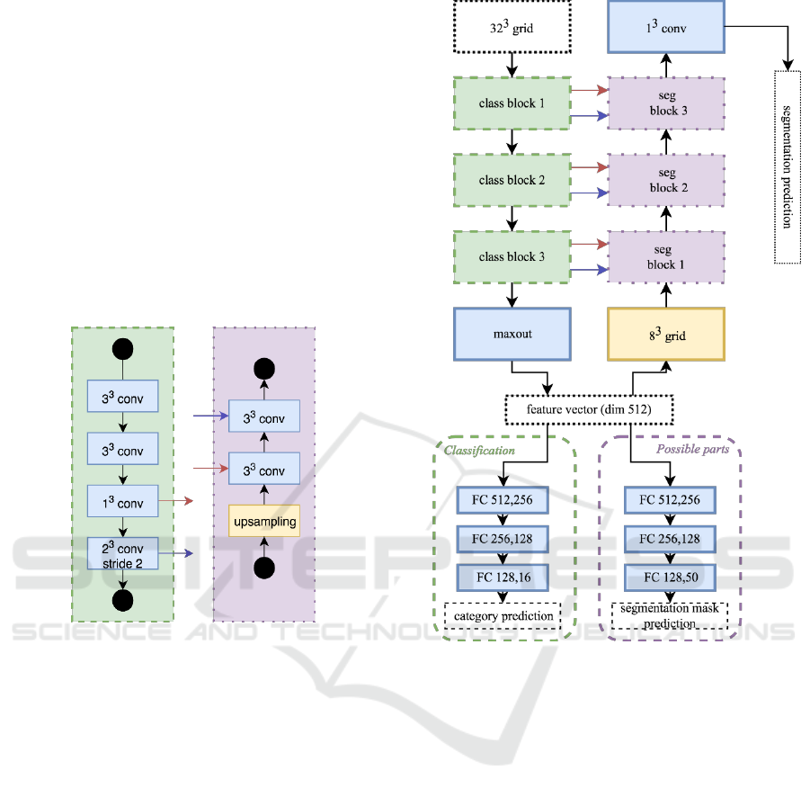
The network is composed of two parts:

classification (down-sampling) and segmentation

(up-sampling) as depicted in Figure 2. Each part

consists of three blocks.

a) Classification block b) Segmentation block

Figure 1: Basic building blocks of a) classification on the

left, and b) segmentation layer on the right.

The main building block of the classification part

of our network is shown in Figure 1 a). We apply two

3D convolutions with zero padding to keep the

dimensions of the input, which are followed by batch

normalization. The results are then concatenated, and

convolution of size 2

with stride 2 is applied to half

the resolution of the input grid.

After each convolution, we use batch

normalization (Ioffe and Szegedy, 2015) and dropout

(Srivastava et al., 2014). ReLU (Nair and Hinton,

2010) activation function is used for the classification

part, and softplus (Zhao et al., 2018) for the

segmentation (except for the last prediction layers).

After the third classification block, we use maxout

(Goodfellow et al., 2013) to convert the grid into a

one-dimensional vector of size 512, which is fed into

the classification multilayer perceptron (MLP) and

softmax layer. We also use the feature vector to

estimate mask for all possible object parts.

Figure 2: Architecture of our U-net neural network with

category prediction and segmentation.

The feature vector is tiled into a grid of size 83 which

is the input into the segmentation part. The

segmentation part of the network uses blocks as

depicted in Figure 1 b). The first convolution of

segmentation block down-samples the number of

channels to the half of the input voxel grid, i.e. with

the input number of channels C

, and C

channels from

skip connection we have C

filters of size C

/2.

The following segmentation block uses the up-

sampled grid from previous block. If not said

otherwise, we also zero-pad the input grid to keep its

dimensions.

As there will always be a loss of information when

up-/down-sampling, we try to compensate this by

using skip connections. We add output of the strided

convolutions right before up-sampling and output of

convolution right after up-sampling.

On Improving 3D U-net Architecture

651

3.2 Implementation Details

Our network is implemented using TensorFlow

(Abadi et al., 2015). We use Adam optimization

(Kingma and Ba, 2014) to minimize sum of softmax

cross entropies – sum over segmentation, sum over

possible mask, and sum over category. We also

multiply the input segmentation by the occupancy

grid, so that the network focuses on minimizing valid

voxels. We use the Adam optimization with an initial

learning rate of 0.0001 and batch size of 16. We

decrease the learning rate by 0.75 each five epochs.

The network generally converges around the 10

epoch with batch normalization. We also apply

gradient clipping in range <-1,1>. Each layer is

followed by dropout layer with keep probability 75%.

4 EXPERIMENTS

The performance of our network has been evaluated

on two different applications – object classification

and part segmentation. In this chapter, we describe

data used, our baseline network, changes to the

architecture, and report how they affect the training

and network generalization.

4.1 Metrics

For comparison of part segmentation results we use

weighted average Intersection over Union (IoU) as

provided by (Yi et al., 2016). Per category average

IoU is computed for each category first by averaging

across all parts of all shapes with the certain category

label. The overall average IoU is then computed

through a weighted average of a per-category IoU.

The weights are the number of samples in each

category. To compare ourselves on object

classification task we use per instance accuracy on

ModelNet (Wu et al., 2015).

4.2 Datasets

For object classification we use two variants of

ModelNet (Wu et al., 2015), i.e. ModelNet40 and its

subset ModelNet10. The ModelNet40 contains

13,834 objects from 40 different categories, where

9,834 are used as training samples and 3,991 as the

test samples. ModelNet10 has 2,468 training samples

and 909 test samples. Since the original ModelNet

contains models represented by edges and vertices,

we use pre-generated dataset of point clouds from

authors of PointNet++ (Qi et al., 2017), where each

model is uniformly sampled by 10,000 points.

For the part segmentation task, we use

ShapeNetPart dataset (Yi et al., 2016). It contains

16,881 objects in 16 categories, represented as point

clouds. Each object consists of 2 to 6 parts with 50

parts in total, where an object does not need to have

all category parts. We use the formal split, where

dataset is split into 12,137 objects for the train set,

1,870 objects for the validation set, and 2,874 objects

for the test set.

4.3 Baseline Network

We based our network on the standard 3D U-net

architecture. The baseline network has similar

structure to network depicted in Figure 2. However,

each block consists of two 3

convolution layers

followed by max pooling instead of 2

convolutions

with stride 2. The baseline also uses convolution 4

instead of maxout. The filter output size is

(32,64,128) for the classification blocks and

(256,128,64) for the segmentation blocks. The

baseline network has ~13.3M trainable parameters

and uses only ReLU as activation function.

With the baseline and no modifications to the

dataset we were able to reach 78.8% IoU. However,

the training suffered from category imbalance (Figure

4) because the network tends to overfit on categories

with higher number of samples. We discuss the

problem in the following sections.

4.4 Removing Max Pooling

As max pooling can lead to the loss of information,

we tried to replace max-pooling layers with

convolution layers of size 2

and stride 2. They halve

the resolution and double the number of channels.

This made the training more stable, but increased the

number of trainable parameters to ~19.5M, where

most of it was contributed by the 4

convolution, that

was used instead of the maxout layer in Figure 2.

Replacing the max pooling raised the IoU to 80.5%.

Though this increased the overall performance,

the network still fails at small parts as thin straps, or

very low-detailed transitions such as gas tank/saddle

and motorbike body, or transition between the tip and

the rest of the rocket. Ground truth for these

categories is shown in Figure 3.

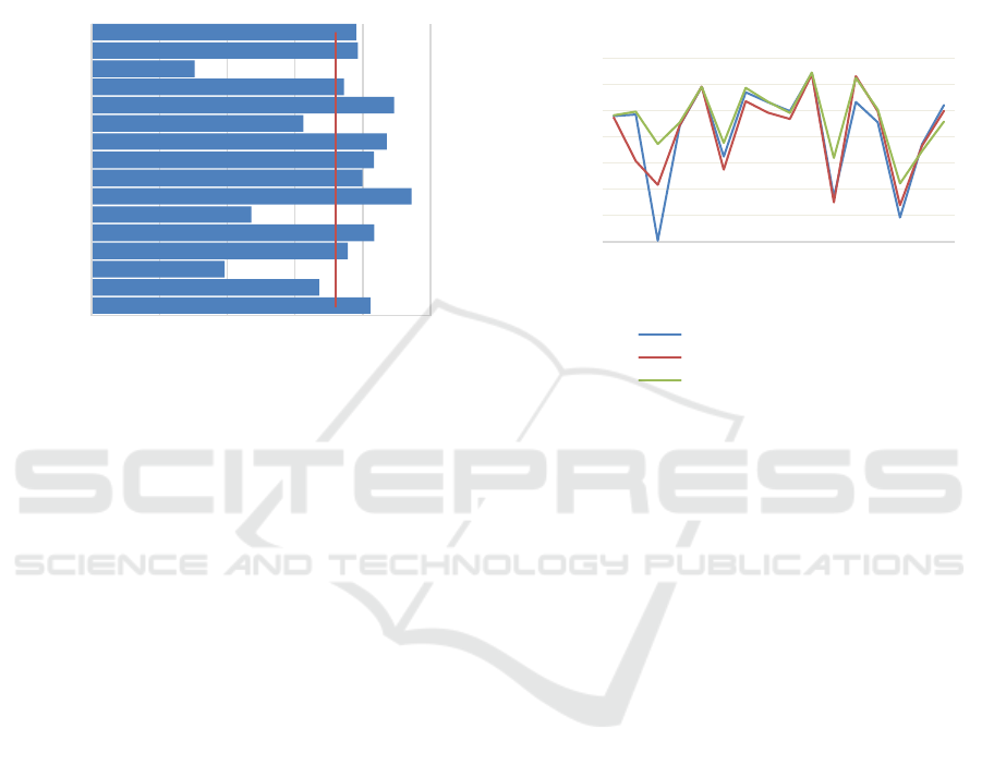
4.5 Category Imbalance

As shown in Figure 4, the ShapeNetPart dataset

suffers from category unbalance, where in the train

set table category has 100 times more samples than

the cap category. As such, the network is likely to

ICSOFT 2019 - 14th International Conference on Software Technologies

652

learn more on these large categories, because the

accumulated loss will be higher for the large

categories. The same goes for the test set, where the

categories table, chair, and airplane contribute to the

result by 65%. Figure 5 shows how can large

categories influence the weighted IoU in comparison

to the average.

Figure 3: Ground truth for problematic categories - bag,

earphones, rocket, and motorbike. Especially, the red strap

for the bag (top left), green straps for the earphones (top

right), green tip of a rocket (bottom right), and motorbike

parts except the yellow body (bottom left) are often

misclassified as neighbouring parts.

We considered simple weighting based on the

distribution of the data, but given the fact that for

large categories the value is close to zero and for

small categories it is evenly distributed, it did not

significantly change the training. As the simple

weighting did not help, we tried to apply probabilistic

weights, which is discussed in the following section.

4.6 Probabilistic Weights

Softmax function takes the input vector and

normalizes the sum of the vector to 1 where each

element is in range <0,1>. Given these properties, it

can also be interpreted as a probabilistic distribution

saying how likely is each part.

We use these probabilities to weight the output of

the softmax cross entropy loss function by (2-P),

where P is the estimated probability of the correct

label. This way the voxels with lower probability

have higher impact on the training. Even though it

improved the overall IoU, it did not solve the problem

with category imbalance.

Weighting also proved to have a regularization

effect, lowering the variance between test and train

data. When weighting was not used the cost and

accuracy on the train set would decrease and increase

respectively, but the accuracy on the test data was

decreasing as the network started to overfit. With the

weighting applied the network tries not to favour any

voxel and thus slowing the overfitting process. In

respect to the backpropagation the weighting works

as additional max term for the correct label whereas

Figure 4: Number of samples per category. ShapeNetPart

training (blue) and test (red) data sample distribution among

the 16 categories.

the loss itself maximizes the difference between

correct label and the others.

Though the network learned better on the hard

categories like cap, rocket, or motorbike, it did not

improve the weighted average IoU.

4.7 Oversampling

When using random permutation of the dataset for

each training epoch, the final result depends on the

luck of the draw, i.e. when the small categories are

not in one of the last batches, their IoU drastically

drops. This can be seen in Figure 6, where the blue

line shows weighted average IoU with value of 82%.

However, the categories with high number of samples

contribute to the overall IoU the most, and as such

there is a significant drop in harder categories like

cap, motorbike, or rocket.

To prevent this behaviour, we oversample the

training set so that each category contains the same

number of samples as the largest category, and each

batch has exactly one sample from each category.

We trained the network again but with

oversampling. For comparison, we took this newly

trained model and compared it with a network trained

without oversampling, but having similar IoU.

The results comparing training with/without the

oversampling are shown in Figure 6, red without

oversampling and green with oversampling. Both

500

1000

1500

2000

2500

3000

3500

4000

4500

5000

Airplane

Bag

Cap

Car

Chair

Earphone

Guitar

Knife

Lamp

Laptop

Motorbike

Mug

Pistol

Rocket

Skateboard

Table

Train set distribution Test set distribution

On Improving 3D U-net Architecture

653

these networks do clearly overfit less, however with

oversampling, the network outperforms on the hard

categories (cap, earphone, motorbike, rocket).

Oversampling increases the training time and

prevents the overfitting, but lowers the overall

accuracy reaching 80.9% IoU. As it repeats some

samples multiple times, we tried simple data

augmentation, i.e. rotation and scale of the point cloud.

Figure 5: The influence of largest categories on weighted

IoU. Case when the three largest categories in test set, as

can be seen in Figure 4 (table, airplane, chair), keeps the

weighted IoU on 82% even though the average is lower –

72% marked in graph by red solid line.

When compared with weighting, data augmentation

had better regularization effect, and got the IoU at

maximum of 82.2%, whereas with the weighting it

reached its maximum at 80.8%.

4.8 Segmentation Mask

Convolutional neural networks are good at finding the

overall structure of the input data, but do not handle

well correct placement of each respective parts often

thanks to the max pooling, i.e. it does not matter

where the eye in the face is as long as it is there.

We tried to leverage the category classification

capabilities by converting the predicted category into

a mask to remove category misclassifications as the

network can reach 97.5% category prediction

accuracy on the test data.

We tried two different approaches: a) learn the

mask during training, and b) generate the mask from

predicted category.

As for a) learning the mask, we tried to learn two

different masks – all possible parts for category and

all possible parts for given sample; does not need to

have all category parts like standing/hanging lamp.

Both approaches led to similar results, however

learning mask for given sample yields slightly better

results.

Approach b) gave cleaner results, but category

misclassifications became more apparent. However,

when the category is misclassified most of the voxels

are misclassified as well. Moreover, most of the parts

are misclassified in its own category, except

categories like cap, rocket, earphone, and lamp,

Figure 6: Comparison of evaluation on the test set, when

trained with and without oversampling. For this

comparison, learned models with similar wIoU are used.

The network model used is the variant of baseline

architecture with convolutions instead of max pooling.

where significant number of voxel misclassifications

is in different category. As such, masking out the

segmentation results as postprocess seems like a valid

strategy that does not introduce too much

inaccuracies when applied on not-fully trained

network.

Though the IoU was not improved, when we

compared confusion matrices, the misclassifications

were more focused in the categories themselves.

4.9 Segmentation Results

As the network has large number of trainable

parameters, where most of them are from the last

down-sampling layers, we replaced the last

convolution with maxout (Goodfellow et al., 2013)

lowering the number of trainable parameters to

~11.1M without affecting the performance.

The network can be trained in 16 hours with inference

time of 20ms per sample. We use

augmentation, oversampling, and learn the

segmentation mask, though we don’t apply the mask.

We also tried various activation functions for the

72,01%

0 20 40 60 80 100

Airplane

Bag

Cap

Car

Chair

Earphone

Guitar

Knife

Lamp

Laptop

Motorbike

Mug

Pistol

Rocket

Skateboard

Table

Per-category IoU (%)

100

Airplane

Bag

Cap

Car

Chair

Earphone

Guitar

Knife

Lamp

Laptop

Motorbike

Mug

Pistol

Rocket

Skateboard

Table

Per-category IoU (%)

82% IoU, no oversampling

80.8% IoU, no oversampling

80.9% IoU, oversampling

ICSOFT 2019 - 14th International Conference on Software Technologies

654

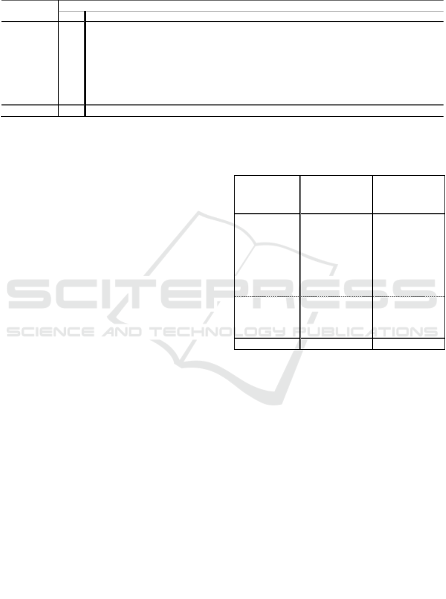
Table 1: Object part segmentation results on ShapeNetPart dataset.

segmentation part with softplus function (Zhao et al.,

2018) yielding best results.

We present our results in Table 1, where we

compare our results with the state-of-the-art methods

for object part segmentation. It can be seen that our

network falls behind most of the architectures. Our

network suffers from having not enough local

information. However, simply increasing the

resolution of the input voxel grid doesn’t improve the

results: doubling the resolution slightly lowered the

accuracy. To improve the local information, we tried

to change the input to a vector per voxel, where the

vector is composed from directions from the voxel

mean to k-nearest points. Though not yielding notable

results, the voxel grid could serve as a look-up table

for other methods struggling with global structure

encoding.

4.10 Classification Results

The network used for tests on ModelNet10 and

ModelNet40 was the same network as depicted in

Figure 2 although we stripped the network of all parts

that are required for segmentation. Resulting network

has ~2.2M trainable parameters. With oversampling

and augmentation, the training time per sample is

25ms and inference time is 3ms. We trained the

network on ModelNet10/40 with batch size of 40. The

network can be trained in 12 hours on ModelNet40.

As shown in Table 2, we compare ourselves with

other approaches also used for segmentation.

Moreover, we include 3DShapeNets (Wu et al., 2015)

since they use a voxel grid as an input and

RotationNet (Kanezaki et al., 2018) as the best

reported result on Princeton ModelNet.

To the best of our knowledge, we outperform or

match most of the existing solutions for object

classification using voxel grids, although each

network was fine-tuned on different type of

application. However, in comparison with

architectures working on other data structures our

approach does not reach notable results.

Table 2: Object classification results on ModelNet10 and

ModelNet40 for methods using point cloud, voxel grid, Kd-

tree, octree, or self-organizing map as an input. Networks

using voxel grids are listed under the dashed line.

5 CONCLUSION

In this paper, we had presented modifications to

3D U-net architecture and in the series of experiments

shown their influence on the training process and

ability to generalise. We show improvements from

the baseline architecture by 3% on the segmentation

task. As voxel grids provide hierarchical global

information, we see a promising way to further

improve the voxel-based architectures by combining

it with approaches focused more on local features, or

with refinement methods.

ACKNOWLEDGEMENTS

This work is supported by Ministry of Education,

Youth and Sports within the project Key technologies

for Time-Of-Flight sensor data processing and

Method

Intersection over Union (IoU)

Mean

air.

bag

cap

car

chair

ear.

gui.

knife

lamp

lap.

motor

mug

pistol

rocket

skate

table

Kd-Net

82.3

80.1

74.6

74.3

70.3

88.6

73.5

90.2

87.2

81.0

94.9

57.4

86.7

78.1

51.8

69.9

80.3

PointNet

83.7

83.4

78.7

82.5

74.9

89.6

73.0

91.5

85.9

80.8

95.3

65.2

93.0

81.2

57.9

72.8

80.6

SO-Net

84.9

82.8

77.8

88.0

77.3

90.6

73.5

90.7

83.9

82.8

94.8

69.1

94.2

80.9

53.1

72.9

83.0

PointNet++

85.1

82.4

79.0

87.7

77.3

90.8

71.8

91.0

85.9

83.7

95.3

71.6

94.1

81.3

58.7

76.4

82.6

SpiderCNN

85.3

83.5

81.0

87.2

77.5

90.7

76.8

91.1

87.3

83.3

95.8

70.2

93.5

82.7

59.7

75.8

82.8

SGPN

85.8

80.4

78.6

78.8

71.5

88.6

78.0

90.9

83.0

78.8

95.8

77.8

93.8

87.4

60.1

92.3

89.4

O-CNN+CRF

85.9

85.5

87.1

84.7

77.0

91.1

85.1

91.9

87.4

83.3

95.4

56.9

96.2

81.6

83.5

74.1

84.4

PointCNN

86.1

84.1

86.5

86.0

80.8

90.6

79.7

92.3

88.4

85.3

96.1

77.2

95.3

84.2

64.2

80.0

83.0

Ours

82.2

77.7

84.4

84.2

76.6

88.7

76.0

88.1

82.3

81.4

94.6

68.0

95.1

81.5

52.5

70.9

78.7

Method

ModelNet40

Classification

Accuracy

ModelNet10

Classification

Accuracy

PointNet

89.2

PointNet++

91.9

Kd-Net

91.8

94.0

O-CNN

90.6

SO-Net

93.4

95.7

SpiderCNN

92.4

PointCNN

84.5

91.0

RotationNet

97.3

98.5

3DShapeNets

77.0

83.5

binVoxNetPlus

85.5

92.3

VoxNet

ORION

93.8

Ours

88.8

93.0

On Improving 3D U-net Architecture

655

visualization (LTACH17013). The authors

acknowledge the support of the OP VVV MEYS

funded project CZ.02.1.01/0.0/0.0/16_019/0000765

„Research Center for Informatics“.

REFERENCES

Abadi, M. et al., 2015. TensorFlow: Large-Scale Machine

Learning on Heterogeneous Systems.

Çiçek, Ö. et al., 2016. 3D U-Net: learning dense volumetric

segmentation from sparse annotation. In Medical Image

Computing and Computer-Assisted Intervention –

MICCAI 2016., pp.424-432.

Goodfellow, IJ. et al., 2013. Maxout Networks. In

Proceedings of The 30th International Conference on

Machine Learning.

Hofmann, D. and Kowshik, B., 2018. Meet RoboSat - End-

to-end feature extraction from aerial and satellite

imagery. [online] Available at:

https://blog.mapbox.com/meet-robosat-af42530f163f

[Accessed 25 Feb. 2019].

Ioffe, S. and Szegedy, C., 2015. Batch Normalization:

Accelerating Deep Network Training by Reducing

Internal Covariate Shift. International Conference on

Machine Learning., pp.448-456.

Kanezaki, A., Matsushita, Y. and Nishida, Y., 2018.

RotationNet: Joint Object Categorization and Pose

Estimation Using Multiviews from Unsupervised

Viewpoints. In 2018 IEEE/CVF Conference on

Computer Vision and Pattern Recognition., pp.5010-

5019.

Kingma, D. P. and Ba, J., 2014. Adam: A method for

stochastic optimization. arXiv preprint

arXiv:1412.6980.

Klokov, R. and Lempitsky, VS., 2017. Escape from Cells:

Deep Kd-Networks for the Recognition of 3D Point

Cloud Models. In 2017 IEEE International Conference

on Computer Vision (ICCV)., pp.863-872.

Li, Y. et al., 2018. PointCNN: Convolution On X-

Transformed Points. In Advances in Neural Information

Processing Systems., pp.828-838.

Li, J., Chen, BM. and Lee, GH., 2018. SO-Net: Self-

Organizing Network for Point Cloud Analysis. In 2018

IEEE/CVF Conference on Computer Vision and

Pattern Recognition., pp.9397-9406.

Maturana, D. and Scherer, S., 2015. VoxNet: A 3D

Convolutional Neural Network for real-time object

recognition. In 2015 IEEE/RSJ International

Conference on Intelligent Robots and Systems (IROS).,

pp.922-928.

Milletari, F., Navab, N. and Ahmadi, SA., 2016. V-Net:

Fully Convolutional Neural Networks for Volumetric

Medical Image Segmentation. In 2016 Fourth

International Conference on 3D Vision (3DV)., pp.565-

571.

Nair, V. and Hinton, GE., 2010. Rectified Linear Units

Improve Restricted Boltzmann Machines. In

Proceedings of the 27th International Conference on

Machine Learning., pp.807-814.

Qi, C. R. et al., 2017. PointNet: Deep Learning on Point

Sets for 3D Classification and Segmentation. In 2017

IEEE Conference on Computer Vision and Pattern

Recognition (CVPR)., pp.77-85.

Qi, C. R. et al., 2016. Volumetric and Multi-view CNNs for

Object Classification on 3D Data. In 2016 IEEE

Conference on Computer Vision and Pattern

Recognition (CVPR)., pp.5648-5656.

Qi, C. R. et al., 2017. Pointnet++: Deep hierarchical feature

learning on point sets in a metric space. In Advances in

Neural Information Processing Systems., pp.5099-

5108.

Riegler, G., Ulusoy, AO. and Geiger, A., 2017. OctNet:

Learning Deep 3D Representations at High

Resolutions. In 2017 IEEE Conference on Computer

Vision and Pattern Recognition (CVPR)., pp.6620-

6629.

Rusu, RB. and Cousins, S., 2011. 3D is here: Point Cloud

Library (PCL). In 2011 IEEE International Conference

on Robotics and Automation., pp.1-4.

Sabour, S., Frosst, N. and Hinton, GE., 2017. Dynamic

Routing Between Capsules. Neural Information

Processing Systems., pp.3856-3866.

Srivastava, N. et al., 2014. Dropout: a simple way to prevent

neural networks from overfitting. Journal of Machine

Learning Research. 15(1), pp.1929-1958.

Su, H. et al., 2015. Multi-view convolutional neural

networks for 3d shape recognition. In Proc. ICCV.

Wang, PS. et al., 2017. O-cnn: Octree-based convolutional

neural networks for 3d shape analysis. ACM

Transactions on Graphics (TOG). 36, p.72.

Wang, W. et al., 2018. SGPN: Similarity Group Proposal

Network for 3D Point Cloud Instance Segmentation. In

2018 IEEE/CVF Conference on Computer Vision and

Pattern Recognition., pp.2569-2578.

Wu, Z. et al., 2015. 3D ShapeNets: A deep representation

for volumetric shapes. In 2015 IEEE Conference on

Computer Vision and Pattern Recognition (CVPR).,

pp.1912-1920.

Xu, Y. et al., 2018. SpiderCNN: Deep Learning on Point

Sets with Parameterized Convolutional Filters.

european conference on computer vision., pp.90-105.

Yi, L. et al., 2016. A Scalable Active Framework for Region

Annotation in 3D Shape Collections. SIGGRAPH Asia.

Zhao, H. et al., 2018. A novel softplus linear unit for deep

convolutional neural networks. Applied Intelligence.

48(7), pp.1707-1720.

ICSOFT 2019 - 14th International Conference on Software Technologies

656