Seamless Development of Robotic Applications using Middleware and

Advanced Simulator

Burtin Gabriel

, Bonnin Patrick

and Malartre Florent

4D-Virtualiz, 10 Allee Evariste Galois, Clermont-Ferrand, France

LISV, Universite de Versailles St Quentin, 10-12 Avenue de l’Europe Velizy, France

Keywords:

Robotic Simulation, Real-time Simulator, Hardware In the Loop, Camera-lidar Sensor Fusion.

Abstract:

This paper addresses the issue of efﬁcient transition from robotic simulation to ﬁeld experiments and valida-

tion. The idea to ease this transition is to proceed step by step with small increments in complexity. A user

begins with a simple and not so realistic simulation and evolve slowly to a complex and realistic one. We

identiﬁed two axis to be tackled to achieve this steps by step complexity. The ﬁrst axis is about the com-

munication with the sensors: each sensors have a speciﬁc protocol. A simple simulation can by-pass this

protocol by proposing a (universal) middleware connection while a complex one will emulate the real pro-

tocol to ensure a realistic data exchange between the processing unit and the sensor. The second axis is the

opportunity to emulate a large spectrum of simulation complexity for a given sensor/environment. To increase

the realism, similarly to the communication protocol, the realism of the sensor and its interactions with the

environment can be increased from simple to the most realistic. These concepts are tested with a real use-case:

the development of an indoor real-time localization system. The main development is done with a simulator

compliant with our requirements. Afterward, the code designed with simulation is tested with a real robot for

ﬁnal validation.

1 INTRODUCTION

The use of simulation for robotics applications valida-

tion is a very actual topic with the rise of autonomous

cars and their authorization to roam free on our roads.

Using a simulator is an interesting option to reduce

the number of kilometers traveled with the real vehi-

cle. Before an autonomous car or robot hits the mar-

ket, several steps has to be overcome. While every-

thing begins with problems and ideas to solve them,

it appears that simulation is an interesting tool for

this matter. Indeed, researchers and companies need

tools to efﬁciently try out and prove ideas/theories to

be converted to industrial goods (Ivaldi et al., 2014).

Usually, both make use of simulator to reduce simul-

taneously duration and development costs. The use of

simulation can sound like a simple and easy improve-

ment but several issues arise when using simulation

to address a problem. Technological locks are block-

ing the smooth transition between simulated and real

world. The main locks are: seamless re-use of the

developed source code, complexity of the simulated

scenarios and pertinence of the simulation compared

to real-world.

First of all, we will deﬁne proposed features

needed for an advanced robotic simulator. Then we

will present a robotic related issue we solved using

simulator (Burtin et al., 2016) compliant with those

features. In the end, we will show and comment the

results obtained both in simulated and real environ-

ments with robots equipped with sensors. Finally, we

will conclude on the effectiveness of the presented

features for the developments of this robotic applica-

tion.

2 APPROACH

To develop a suitable simulation tool aiming at val-

idating a speciﬁc scientiﬁc concept, we previously

need to identify the steps involved in the develop-

ment of the concept. As seen in the ﬁgure 1, the loop

is the most time consuming step: we have to do an

unknown number of loops to improve incrementally

the solution and every loop needs experiments. This

experiment step can be done using simulation during

the early loops, and possibly until second to last be-

Gabriel, B., Patrick, B. and Florent, M.

Seamless Development of Robotic Applications using Middleware and Advanced Simulator.

DOI: 10.5220/0007831002390246

In Proceedings of the 9th Inter national Conference on Simulation and Modeling Methodologies, Technologies and Applications (SIMULTECH 2019), pages 239-246

ISBN: 978-989-758-381-0

239

fore the real world experiment (last loop). During

these loops, the goal is to increase the complexity and

solve issues alongside for an interesting conclusion

and possibly innovation.

Figure 1: Steps involved in the scientiﬁc method.

2.1 Universal Interface

The ﬁrst time related issue with innovation is the du-

ration needed to perform the adaptation of the source

code between different simulation platforms (Stara-

nowicz and Mariottini, 2011). This transition usually

implies a radical change in programming language

and communication protocols with the simulated sen-

sors resulting in a new driver to implement. Some-

times, the source code has to be entirely re-written to

change the programming language (for example mat-

lab toward C/C++). ROS (Robotic Operating Sys-

tem), a robotic designed middleware allowed a much

more homogeneous format in data transfer and com-

munications: every data can be sent on the network

whatever is the original sensor and received by a ROS

node. Gazebo (Koenig and Howard, 2004) is an open-

source simulator developed within the ROS commu-

nity, it has a fully ROS compatible interface. How-

ever it still needs nevertheless somebody to develop

the ROS driver for the real sensor’s driver to be com-

patible with ROS when doing the transition to real

sensors. The researcher is prone to change its sim-

ulation platform to increase the complexity of the ex-

periment because all simulators have speciﬁc ranges

of realism. By making sure it has a full compatibility

with every middleware (Ardiyanto and Miura, 2012),

a simulator may not force the user to change its code

if he changes between middleware compatibles simu-

lation platforms. For example, V-REP (Rohmer et al.,

2013) is another ROS compatible simulator that al-

lows a ROS program to be tested with, even if it was

previously tested with Gazebo. During the ﬁnal tests

of the code, developers has to take into account the

real sensor and the computation platform on which

the code will run. They will need to be able to get

rid of any middleware and take into account the real-

ity of the sensor and interface with it through the pri-

vate communication protocol. An advanced simula-

tion platform has to be able to emulate this crucial last

step, vital to be connected to the real sensor during

the real world experiment. In order to perform such

task, the simulator needs to be able to emulate the

data frame produced by the sensor and its ﬁrmware

and transmit it with the same physical support (Serial,

Ethernet, CAN bus). By doing so, the simulator pro-

pose an identical virtual twin for the algorithm to con-

nect to: if the driver is correctly implemented, he can

receive data from the real and virtual sensor without

being able to tell the difference and with no modiﬁca-

tion of the source code.

2.2 Modular Complexity

Obviously, before testing a robot system in a full com-

plex environment, we proceed by incremental steps.

First of all, simple scenarios and if there are any suc-

cesses, the complexity can grow toward the ﬁnal full

scale test. With the same idea, when starting with

a simulation platform, we need to start with a sim-

ple simulation and increase the complexity before the

transition to the real world experiments. Two choices

are available: every time we need higher complexity,

we change the simulation platform to have better re-

alism, or we use a simulator able to emulate a wide

range of complexities by itself. The second option

is preferable because in the case of the ﬁrst one, the

time lost to transfer the code from a simulator to an-

other may be important, but the time lost to learn how

to use the new simulator and create the scenarios is

greater. Considering the second solution, the simu-

lation platform has to be able to produce sensor data

with adjustable realism which means that a single sen-

sors can be declined into several versions of increas-

ing complexity. For example, the most basic sensor

produces perfect measurement without noise/bias. A

more complex version includes a white noise and/or a

bias. The highest and most complex version would

mimic the measurement method of the real sensor,

producing a noise consistent with the environment

and the sensor. This way of thinking can also be ap-

plied to the environment itself to determine the sce-

nario complexity. For example, a basic scenery (mo-

tionless, simple shapes and monochromatic) won’t

produce the same results than a complex one (ani-

mated pedestrians, moving vehicles, realistic shapes

and photo-realistic textures). Besides the geometric

aspect, climate (snow, rain, shadows) can also prove

critical for the behaving of the application and its ﬁnal

result.

SIMULTECH 2019 - 9th International Conference on Simulation and Modeling Methodologies, Technologies and Applications

240

3 ALGORITHM IMPLEMENTED

In order to test the impact of the simulation, we

have developed a localization method from scratch for

man-made indoor robot navigation.

An important hypothesis in our use-case is the fact

that the robot is evolving in a man-made environment,

comparable to an industry (factory) or ofﬁce/hospital

type. We state that the robot will encounter numer-

ous structured elements with strong vertical and hori-

zontal lines. Considering a ﬂat ﬂoor, we also assume

that the movement is only 2D. With this new assump-

tion and the previous one, we can narrow features to

propose a sparse localization method using speciﬁc

landmarks. The most invariant observable elements

in the image, as explained before, are going to be the

vertical lines. 3D horizontal and other more random

lines would have an incidence angle due to the point

of view of the camera and wouldn’t be invariant in the

image, thus inducing more computation to detect and

track them.

Using segments to perform SLAM (Simultaneous

Localisation And Mapping) processing have been ex-

plored either with a lone lidar (Choi et al., 2008) or

camera alone (Zuo et al., 2017). SLAMs are gener-

ally split between sparse and dense vision algorithms.

Sparse SLAMs are using only a few salient features

in the image to compute the localization, for exam-

ple the ORB-SLAM (Mur-Artal et al., 2015). Each

feature is represented and stored speciﬁcally in the

map to be used later as reference in the localization

algorithm. These types of process only need a small

percentage of the pixels from the entire image to be

tracked, while dense methods use almost all the pix-

els. Because dense methods such as DTAM (Dense

Tracking And Mapping)(Newcombe et al., 2011) use

every pixels from the image, users need a powerful

hardware to perform all the operations in real-time.

Most of the time, GPU processing is used to im-

prove the computation speed. RGB-D (Kinect, Xtion)

and depth camera sensors brought new SLAMs sys-

tems (Schramm et al., 2018), with new approaches.

They avoid the issue of initialization from unknown

range for the features. Monocular cameras have the

weakness to be unable, using only one frame, to ob-

tain the distance between an object and the camera

for its given pixel in the image (scale factor). LSD

(Von Gioi et al., 2012) is massively used by monoc-

ular and stereo-vision SLAMs systems (Engel et al.,

2014) or (Pumarola et al., 2017) but this line segment

detector is too generic and extracts all segments avail-

able while processing only B&W images: the pro-

cess is not optimized enough. Moreover, the RGB to

B&W conversion is a potential danger of missing gra-

dients because of the gray level conversion method.

The idea to use both lidar and monocular camera has

been more usually applied to mobile objects detec-

tion and tracking (Asvadi et al., 2016) but more rarely

to localization itself. In our case, we will focus on

the detection of vertical lines in the camera because

they are commonly found and invariant regarding our

environment. The common slam, using these types

of features are commonly referred as ”bearing” only

slam (Bekris et al., 2006), they are proven effective

in minimalist set-ups with simple environments (Zuo

et al., 2017).

In order to extract these vertical segments in the

image (which are supposed to be the projection of 3D

vertical structures of the scene: doors, angles of corri-

dors), we are looking for classical edge segmentation

composed of well known steps (Nachar et al., 2014):

gradient computation, thinning, closing, linking, and

polygonal approximation.

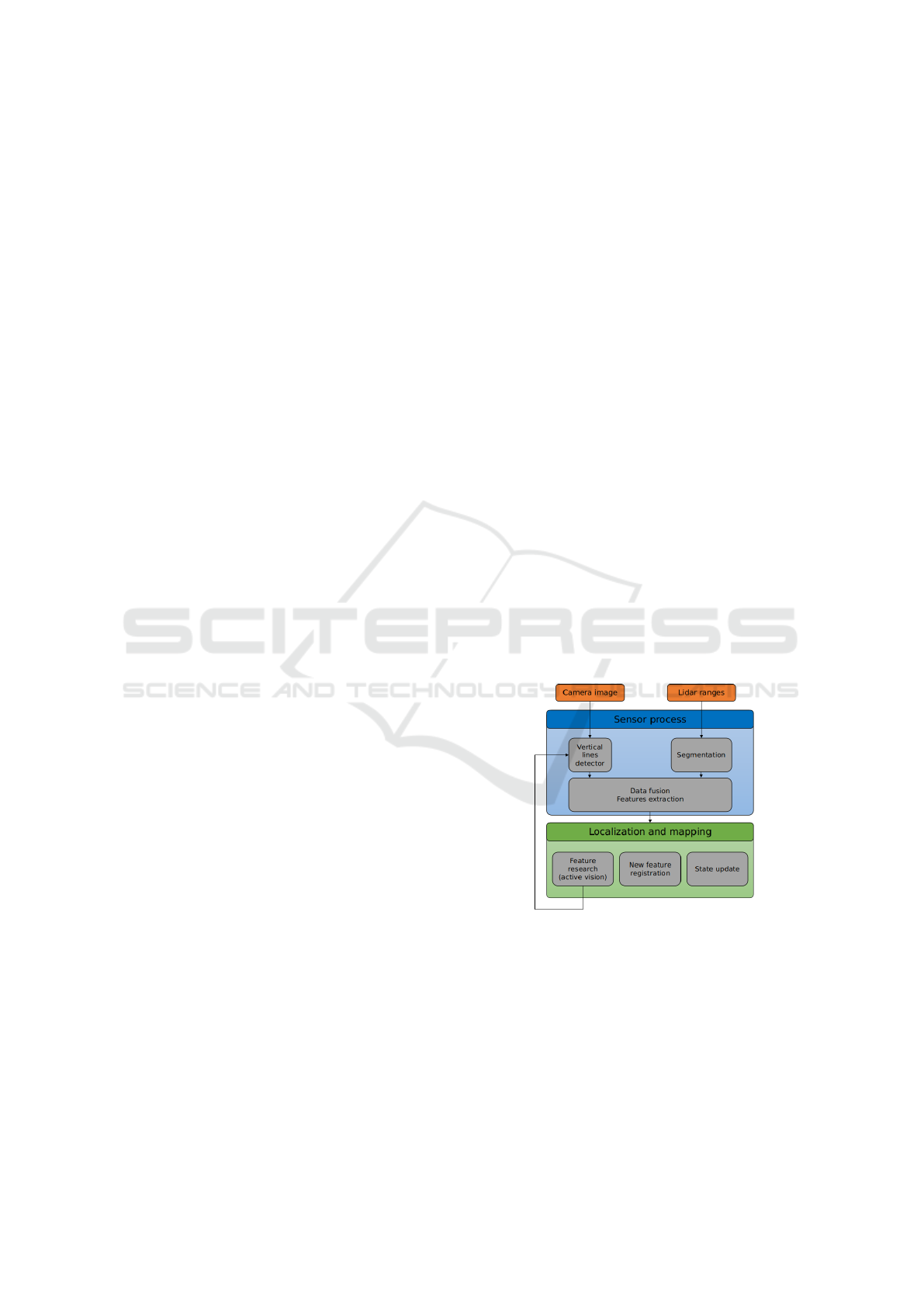
The localization process is an optimized parallel

pipeline able to cross data from the lidar and camera

sensors (Figure: 2). Each data process is split, but

synchronous to use both extracted data at the same

moment during the feature extraction stage. The ob-

jective is to detect a feature and determine its 3D po-

sition in the camera frame. The camera process ex-

tracts vertical lines in the image while the lidar pro-

cess does a segmentation and a time-forward predic-

tion to match the camera’s data time-stamp.

Figure 2: System overview.

The lidar, placed horizontally on the robot, pro-

duces an horizontal plane with the successive dis-

tances measurements. Our lidar process produces,

through the lidar segmentation algorithm, a set of

lines representing the environment around our robot.

The camera, located above the lidar, through the lines

detection algorithm, extracts a set of vertical lines in

the focal plane of the image. The fusion of both of

these data gives us a set of 3D points in the camera

frame (Figure: 3).

Seamless Development of Robotic Applications using Middleware and Advanced Simulator

241

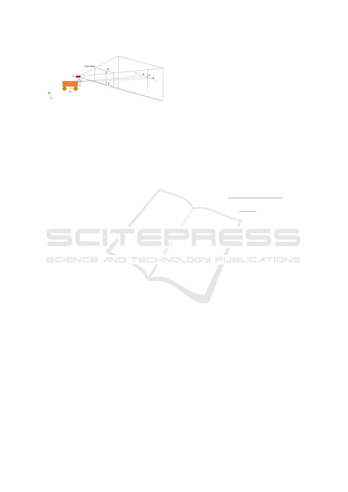
Figure 3: Feature (P) detected in the focal and lidar plane.

First we will see the optimized vertical lines de-

tection algorithm for images processing. Then we

will develop the 3D points extraction process using

the camera vertical features and the horizontal lines

from the lidar process. In the end, we will propose

a SLAM implementation using the extracted features

from the previous processes.

3.1 Lidar Process and Fusion

In this section, we will quickly explain the lines ex-

traction from lidar’s data and their fusion with fea-

tures previously extracted from the image.

In a former work, we applied Wall-Danielsson

to the lidar pointcloud (Burtin et al., 2018). This

method, originally used in the vision ﬁeld, was found

to be efﬁcient at segmenting lidar data very fast and

accurately.

Those lines computed previously in the polygonal

approximation exist in the 2D plane deﬁned by the

lidar’s lasers. Therefore, we can compute the coordi-

nates of these lines in the camera frame with the ex-

trinsic parameters (homogeneous transformation ma-

trix between lidar and camera frames).

The image process provides us vertical lines in the

focal plane of the camera. We can compute from each

line a 3D plane (CDE) (cf. Figure: 3) composed of

the line segment (DE) and the focal point of the cam-

era (C).

The objective is to compute the intersection be-

tween a 3D plane and a 3D line extracted from the

camera and lidar data. This solution is assured to be

unique and existing because (AB) is not coplanar nor

collinear with (CDE) plane.

It’s important to note that points A and B are pro-

jected in the camera frame at the exact moment the

image is taken. Because the lidar and camera have

different frame rates, data aren’t synchronized and are

generated at different moments.

To tackle this issue, we apply a rigid transforma-

tion, composed of two :

1. The prediction of the would-be lidar’s measure,

considering the current velocities and the time

step between the lidar and the camera data;

2. The rigid transformation between lidar and cam-

era frame;

3.2 Localization using a SLAM Method

The extracted features are 3D points, but with our hy-

pothesis of planar environment we can make a 2D as-

sumption. 3D features become 2D and we can deﬁne

them in the camera frame with cartesian (x

, y

) or po-

lar coordinates.

We decided to implement a SLAM system using

an extended Kalman ﬁlter (Kalman, 1960) with the

observations from both the camera and lidar using the

cartesian coordinates. The estimation of the state vec-

tor, including the 2D pose (x

, y

, α

) and the ”n” fea-

tures is 3 + 2 × n long:

= [x

, y

, α

, x

, y

, · · ·, x

, y

] (1)

and the measurement vector, issued by the features in

polar coordinates:







− x

)

+ (y

− y

)

= arctan(

− y

− x

) − α

(2)

Our evolution model estimates the pose of the robot at

the next step with the evolution function f taking

the state vector, and

, the command applied to the

robot, as parameters:

k+1

= f(X

, u

) + q

(3)

is a Gaussian, white noise with zero-mean, repre-

sentative of the evolution noise.

The four steps of the Kalman algorithm are: Pre-

diction, Observation, Innovation and Update.

4 VIRTUAL ENVIRONMENT

One of the sides objectives in developing this local-

ization method was the development, use and vali-

dation of an advanced robotic simulator. The con-

cerned simulator is 4DV-Sim, developed by the com-

pany 4D-Virtualiz. Its development was initiated by

two robotic PhD students (perception and command

ﬁelds), that needed a powerful and capable simula-

tor to speed up their work. At the end of their thesis,

they patented the simulator and created a company. It

has become a professional tool dedicated to real-time

robots simulation in an HIL (Hardware In the Loop)

manner. The aim of this simulator is to replicate very

accurately real environments, sensors and robots into

the virtual world, including shadows, textures, geo-

referencing, communication protocols, disturbances,

etc (Figure: 4).

SIMULTECH 2019 - 9th International Conference on Simulation and Modeling Methodologies, Technologies and Applications

242

(a) Real sensors

(b) Virtual sensors

Figure 4: Comparison of Camera, GPS ans LIDAR sensors

between real data and data produced with the 4DV-Sim sim-

ulator.

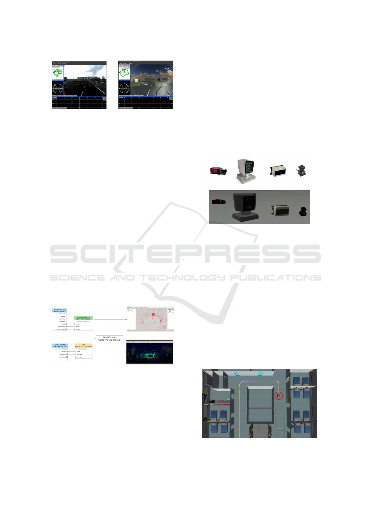
4.0.1 Universal Interface and Modular

Complexity

The simulator is designed to be able to connect in-

dependently to a middleware (ROS, RT-Maps, etc)

or the proprietary interface. In ﬁgure 5, we can see

on the left two conﬁgurations: on top, the Velodyne

system connected to a ROS interface, on the bottom,

it is connected to the proprietary interface. The re-

sults of the ﬁrst set-up can be seen directly on Rviz,

ROS compatible viewer (top right). The results of

the second set-up can be displayed, either directly

with the Veloview, Velodyne viewer provided by the

company (bottom right), or go through the ROS node

”velodyne-pointcloud” to be converted to a regular

ROS message and seen again on Rviz. The same idea

is therefore applied to every real sensor (2D/3D LI-

DARs, IMU, Camera, Odometers, etc ) implemented

in the simulator: the end-user is able to use it either

with the middleware for preliminary tests or the real

protocol and drivers to prepare for the transition to the

real sensor.

Figure 5: Velodyne sensor with ROS and brand interface

seen on Rviz and Velodyne viewer.

This simulator offers sensors with diverse degrees

of realism: it was possible during early prototyping

to use a ”perfect” LIDAR, providing perfects mea-

sured ranges, without any measurement noise. Later,

when our algorithm obtained appropriate results, we

increased the complexity by adding random Gaussian

measurement noise. Finally, before ﬁeld testing, we

experimented the algorithm with the virtual replica

of the real sensor.The virtual replica has exactly the

same characteristics than the real one: FOV, resolu-

tion, noise measurement, maximum range, frequency,

appearance and the communication protocol. In the

ﬁgure 6, we can observe several real sensors (top) and

their virtual replica. From left to right, we have a Mar-

lin camera, a HDL-64E Velodyne (3D lidar), a LD-

MRS Sick (multi-layer lidar) and an UTM-30LX-EW

Hokuyo (2D lidar).

The simulator is able to work in an HIL (hardware

in the loop) fashion which means that once the source

code is validated with the virtual platform, it can be

instantaneously carried to the real platform to be exe-

cuted without modiﬁcations.

Figure 6: Real and virtual sensors.

The use of a simulator also gives the opportunity

to have exact repeatability to compare the results, ac-

cess to ground truth and produce various datasets with

different environments and robot set-ups, advantages

we do not posses with experiments in real environ-

ment.

4.0.2 Robot Set-up

The simulated robot is a Dr. Robot Jaguar, virtu-

ally equipped with a URG-4LX Hokuyo lidar and a

640x480 global-shutter camera (pinhole model). The

simulated lidar has the same parameters than the real

URG-04LX (min angle, max angle, resolution, fre-

quency, etc.) and the noise added to the measures is

Gaussian distributed with parameters provided by the

factory data-sheet.

Figure 7: Simulated indoor environment containing the

robot (red circle) and command trajectory (yellow).

Seamless Development of Robotic Applications using Middleware and Advanced Simulator

243

(a) Simple

(b) Complex

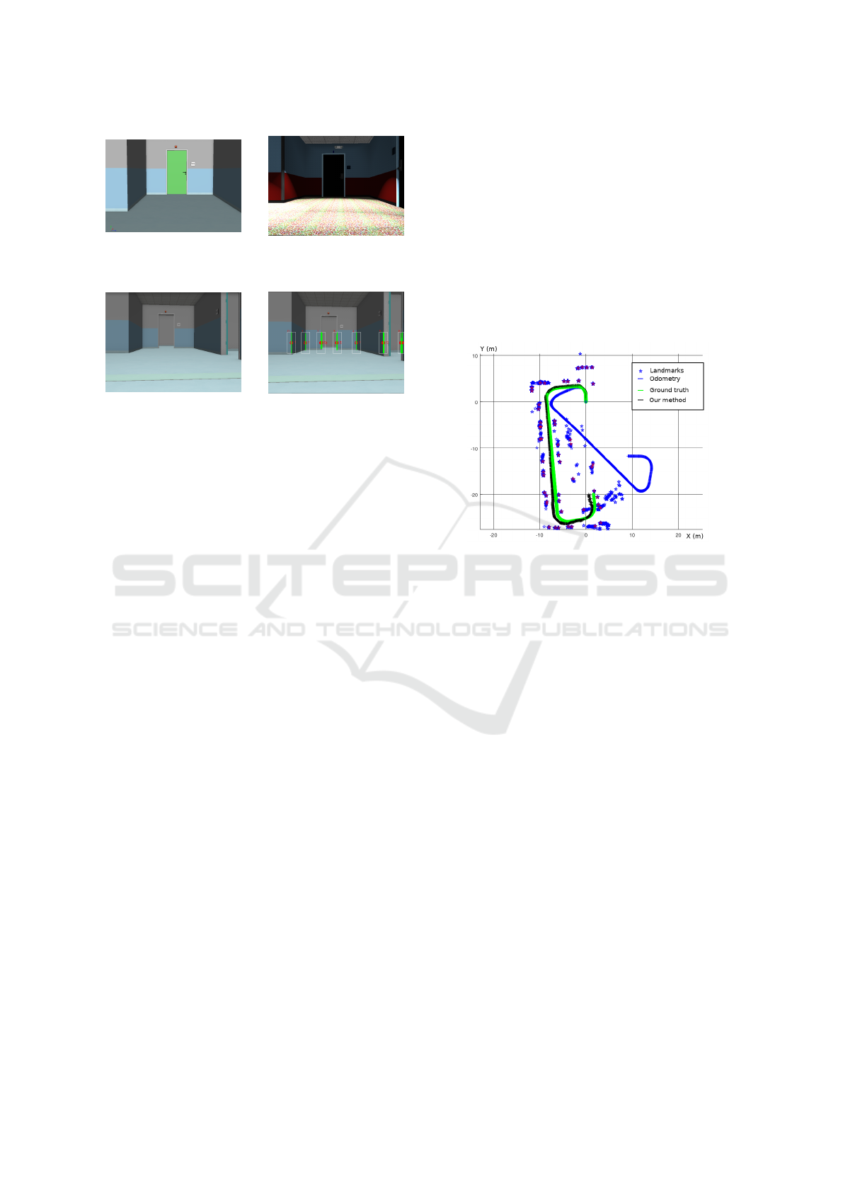
Figure 8: Same environment, different complexity.

(a) Original image

(b) Features

Figure 9: Use of ROI and the 2D features results in the

SLAM map.

The environment we used is a replica of a real

American hospital (Figure: 7). All doors, doorways,

beds, hallways have the right scale and materials ef-

fects. In preliminary work, we used two different sets

of textures and lighting effects to improve gradually

the performance of the vision algorithm (Figure: 8) by

adding more complexity to the scenario, accordingly

to the previously explained method. We will focus the

results produced with the most realistic scenarios.

4.0.3 Localization

We implemented the vertical detector presented pre-

viously and added the lidar data to obtain our 3D fea-

tures. In order to reduce the computation time we

limited the number of detected vertical lines and nar-

rowed this to the lines around the horizon, we can ob-

serve the projection of the 3D extracted features from

the previous image in cooperation with the lidar us-

ing camera intrinsic and extrinsic parameters (Figure:

9b).

The average time needed to extract verticals in

a ROI is 1.6623ms. Using a sparse SLAM system

(even without multi-threading), we can reasonably

track enough features in real time to feed a localiza-

tion process.

We performed our experiments in the simulated

environment using the described robot and setup. The

ﬁnal virtual result is displayed in the Figure: 10. The

blue stars are the extracted and tracked features. One

can recognize the shape of the building shown in top-

view from Figure: 7. The green track is the ground

truth given by the simulator. The blue track is the es-

timated localization using only the odometry of the

robot. We can notice the rapid drift of the odometry

during turns and it’s relative precision during forward

motion. The black track is the estimated position of

the robot using the kalman ﬁlter. The track is split

in two parts, the ﬁrst part has a very precise local-

ization (an average 2cm error relatively to the ground

truth), then a diverging part. The ﬁnal error is 0.3m

over a 40m trajectory. Blue stars are our observed

landmarks and red one are registered in the map cre-

ated. This conclude our virtual tests, considering that

further tests should be on a real robot to conﬁrm the

results.

Figure 10: Localization results.

4.1 Real Experiments

Real experiment were conducted in the hallway of

a public building. We used a Kobuki TurtleBot2

platform with an Hokuyo 04LX and an Intel Re-

alsense D435 placed on the top of the robot. The Re-

alSense sensor is used only to provide a global shutter

640x480 image, we didn’t use the RGB-D feature be-

cause it did not provide depth information with sufﬁ-

cient range and precision (the corner seen on the left

of the hallway is not seen at 3m). The environment

we experienced in is about 40m long, having several

patio doors with large panes, solid doors and shiny

ﬂoor.

The real environment brought additional complex-

ity to the sensors due to two facts: the large win-

dows panes and the ﬂoor that reﬂects the environment.

The ﬁrst issue comes from the sun light that blinds

the LIDAR sensor depending on the intensity of the

rays. The second is brought by the clean plastic ﬂoor

that create ”false” verticals in the image by reﬂecting

lights on the ceiling and doors. The ﬁrst issue was

solved by ﬁltering the LIDAR data while the second

one was only a matter of ROI focusing to exclude mis-

leading verticals.

Our strong initial hypothesis, 2D movement and

camera-lidar rig coplanar to the ﬂoor, is reasonable:

SIMULTECH 2019 - 9th International Conference on Simulation and Modeling Methodologies, Technologies and Applications

244

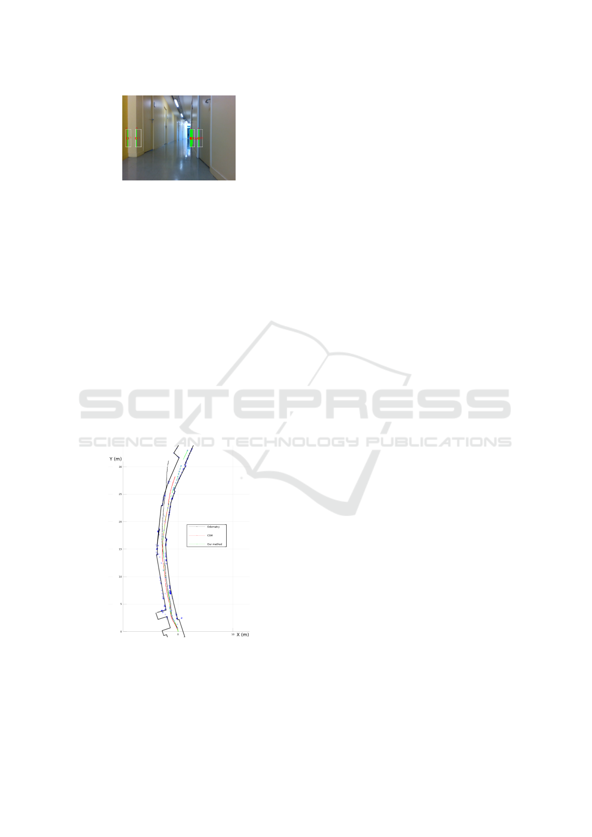
Figure 11: Detections with the real set-up.

even with small angular errors, we still manage to de-

tect vertical lines in our image.

As explained before, we do not have a proper

ground-truth available for real experiment, thus we

can’t know the exact position of the robot during the

experiment but we do have the 2D model of the build-

ing provided by the architects. This model have been

produced using precise (< 1cm) measurement by pro-

fessional surveyors, therefore, we can estimate the ef-

ﬁciency of the robot localization using the compari-

son between the landmarks registered by our system

and the solid shape given by exact model (black shape

in ﬁgure 12).

We compared the localization efﬁciency with an-

other method: the canonical scan matcher (CSM)

(Censi, 2008). We tried the ORB-Slam (Monocular)

but the complex light rendered the initialization im-

possible. Since there is no loop closing in this hall-

way, the CSM should not have particular disadvan-

tage.

Figure 12: Localization results.

On the ﬁgure 12, we can observe the results of

the different methods. The black trajectory is the lone

odometry. The red one is the CSM result. The Blue

stars are the landmarks registered by our method, and

the trajectory is green. The odometry is outside the

building frame but not that much, contrary to the vir-

tual odometry, this one is more precise. This can be

explained by the motion method of the robot: the vir-

tual is a 4 wheeled robot and the TurtleBot is a 2

wheeled. The later present a reduced slippery dur-

ing the turns, thus reducing the error on the odometry

that made the assumption of slip-free rolling condi-

tion. The low range of the LIDAR and narrow FOV

of the camera limits the number of landmarks avail-

able but the algorithm manages to detect several of

them and successfully tracked, even with a complex

lighting. The use of RGB-D sensors to combine the

image and depth with less calibration and more ac-

curate results is an interesting perspective with more

depth range.

5 CONCLUSIONS

In this paper, we proposed an idea of features an ad-

vanced robotic simulator would require. There are

two main features, beside the ability to provide real-

time simulation. The ﬁrst is having multiple inter-

facing capacity to be used at ﬁrst with a middleware

and then with the real sensor protocol. The second

would be the ability of the simulator to provide in-

creasing level of complexity to reduce the gap created

by the transition between simulation and reality. A

real accurate emulation of the sensor (measure, proto-

col, appearance) is a key to have a seamless transition.

We established a use case (robot navigation), built an

extended Kalman ﬁlter to provide fast robot localiza-

tion, re-using sensors data from others purposes. We

evaluated the interest in focused images processing

to reduce the computation time and observed a sig-

niﬁcant improvement, enough to process all features

in real-time on a low grade computer. The early de-

velopments were done using the described simulator,

using ROS to simplify data exchanges and a growing

complexity of simulation. This increment have been

simultaneously focused on the sensor and the envi-

ronment realism to match the ﬁnal test. Our last ex-

periment was performed with real robot and sensors

and we managed to connect to this set-up without any

modiﬁcations in our code. The algorithm worked ”out

of the box” with some parameters tuning and there-

fore, proves the interest in the proposed features.

ACKNOWLEDGMENT

This research was performed within the framework

of a CIFRE grant (ANRT) for the doctoral work of

G.Burtin at 4D-Virtualiz and LISV.

Seamless Development of Robotic Applications using Middleware and Advanced Simulator

245

REFERENCES

Ardiyanto, I. and Miura, J. (2012). Rt components for us-

ing morse realistic simulator for robotics. In The 13th

SICE System Integration Division Annual Conference,

pages 535–538.

Asvadi, A., Girao, P., Peixoto, P., and Nunes, U. (2016). 3d

object tracking using rgb and lidar data. In Intelligent

Transportation Systems (ITSC), 2016 IEEE 19th In-

ternational Conference on, pages 1255–1260. IEEE.

Bekris, K. E., Glick, M., and Kavraki, L. E. (2006). Evalu-

ation of algorithms for bearing-only slam. In Robotics

and Automation, 2006. ICRA 2006. Proceedings 2006

IEEE International Conference on, pages 1937–1943.

IEEE.

Burtin, G., Bonnin, P., and Malartre, F. (2018). Vision based

lidar segmentation for accelerated scan matching. In

Journal of Communications, volume 13, pages 139–

144.

Burtin, G., Malartre, F., and Chapuis, R. (2016). Reduc-

ing the implementation uncertainty using an advanced

robotic simulator.

Censi, A. (2008). An ICP variant using a point-to-line met-

ric. In Proceedings of the IEEE International Confer-

ence on Robotics and Automation (ICRA), Pasadena,

CA.

Choi, Y.-H., Lee, T.-K., and Oh, S.-Y. (2008). A line fea-

ture based slam with low grade range sensors using

geometric constraints and active exploration for mo-

bile robot. Autonomous Robots, 24(1):13–27.

Engel, J., Sch

ops, T., and Cremers, D. (2014). Lsd-slam:

Large-scale direct monocular slam. In European Con-

ference on Computer Vision, pages 834–849. Springer.

Ivaldi, S., Padois, V., and Nori, F. (2014). Tools for dy-

namics simulation of robots: a survey based on user

feedback. arXiv preprint arXiv:1402.7050.

Kalman, R. E. (1960). A new approach to linear ﬁltering

and prediction problems. Transactions of the ASME–

Journal of Basic Engineering, 82(Series D):35–45.

Koenig, N. and Howard, A. (2004). Design and use

paradigms for gazebo, an open-source multi-robot

simulator. In 2004 IEEE/RSJ International Confer-

ence on Intelligent Robots and Systems (IROS)(IEEE

Cat. No. 04CH37566), volume 3, pages 2149–2154.

IEEE.

Mur-Artal, R., Montiel, J. M. M., and Tardos, J. D. (2015).

Orb-slam: a versatile and accurate monocular slam

system. IEEE Transactions on Robotics, 31(5):1147–

1163.

Nachar, R., Inaty, E., Bonnin, P., and Alayli, Y. (2014).

Polygonal approximation of an object contour by de-

tecting edge dominant corners using iterative corner

suppression. VISAPP International Conference on

Computer Vision Theory and Applications, pp 247-

256, Jan 2014, Lisbon, Portugal.

Newcombe, R. A., Lovegrove, S. J., and Davison, A. J.

(2011). Dtam: Dense tracking and mapping in real-

time. In Computer Vision (ICCV), 2011 IEEE Inter-

national Conference on, pages 2320–2327. IEEE.

Pumarola, A., Vakhitov, A., Agudo, A., Sanfeliu, A.,

and Moreno-Noguer, F. (2017). Pl-slam: Real-time

monocular visual slam with points and lines. In

Robotics and Automation (ICRA), 2017 IEEE Inter-

national Conference on, pages 4503–4508. IEEE.

Rohmer, E., Singh, S. P., and Freese, M. (2013). V-rep:

A versatile and scalable robot simulation framework.

In 2013 IEEE/RSJ International Conference on Intel-

ligent Robots and Systems, pages 1321–1326. IEEE.

Schramm, S., Rangel, J., and Kroll, A. (2018). Data fusion

for 3d thermal imaging using depth and stereo camera

for robust self-localization. In Sensors Applications

Symposium (SAS), 2018 IEEE, pages 1–6. IEEE.

Staranowicz, A. and Mariottini, G. L. (2011). A survey and

comparison of commercial and open-source robotic

simulator software. In Proceedings of the 4th Interna-

tional Conference on PErvasive Technologies Related

to Assistive Environments, page 56. ACM.

Von Gioi, R. G., Jakubowicz, J., Morel, J.-M., and Randall,

G. (2012). Lsd: a line segment detector. Image Pro-

cessing On Line, 2:35–55.

Zuo, X., Xie, X., Liu, Y., and Huang, G. (2017). Robust vi-

sual slam with point and line features. arXiv preprint

arXiv:1711.08654.

SIMULTECH 2019 - 9th International Conference on Simulation and Modeling Methodologies, Technologies and Applications

246