Smoothing and Time Parametrization of Motion Trajectories
for Industrial Machining and Motion Control
Kv
ˇ
etoslav Belda
a
Department of Adaptive Systems, The Czech Academy of Sciences, Institute of Information Theory and Automation,
Pod Vodarenskou vezı 4, 182 08 Prague 8, Czech Republic
Keywords:
Path Model, G-Code, Path Smoothing, Time Parametrization, B
´
ezier Curves, Industrial Robotics.
Abstract:
The paper deals with path smoothing and time parametrization procedures intended for motion control of in-
dustrial machine tools and robots. Path smoothing, considered in this paper, is based on the application
of B
´
ezier curves. A possible straightforward solution ensuring compliance with given admissible positional
tolerances is introduced. Consequent time parametrization considered here employs arc length and specific
construction of acceleration polynomials. It describes the motion along the obtained smoothed curve geome-
try. It is given by timing the arc length, thus the construction of the feed rate profile. The key parts of the time
parametrization comprise: computation of path length; time parametrization with respect to arc length; and de-
composition to the individual Cartesian components describing individual curve coordinates. The theoretical
results are presented by representative examples in 2D and 3D spaces.
1 INTRODUCTION
Nowadays, a lot of Computer-Aided Design (CAD)
tools offer a simple way of construction of various
paths and shapes with complicated geometry. This ge-
ometry is usually stored as sets of points and modeled
by a combination of specific parametric curves. One
example of the advanced CAD tools is NX PLM
software (Siemens, 2019), which, with the applica-
tion of industry-oriented modules, offers the option
to store path’s description in specific G-Code used
in Computer Numeric Control (CNC) machine tools
(Xavier et al., 2010). This G-Code can be uploaded
directly to the real control system of a machine tool
or robot to ensure required motion along reference
trajectory.
In G-Code, the geometry data are typically re-
stricted to low level segments such as points (dwell,
fixed positions), straight lines (abscissas, linear seg-
ments) and arcs (circular segments). These restric-
tions lead to huge numbers of linear segments due
to complicated initial curve geometry and several cir-
cular segments for pure circular arcs. Transition be-
tween such segments are contiguous, but not smooth.
In order to satisfy the given kinematic constrains
without having to stop at each point of higher or-
a
https://orcid.org/0000-0002-1299-7704
der discontinuity, the path needs to be smoothed
in a preprocessing procedure before the actual time
parametrization, from which full-featured motion tra-
jectories arise (Zhang et al., 2018). Note that every
stop means increase of working time and increasing
of energy demands on braking and repeated starting
(Othman et al., 2015).
A recent trend in industrial production is to em-
ploy increasingly complicated motion trajectories es-
pecially in the case of industrial robots, see e.g. Fig. 1.
Thus, real-world testing on machine tools becomes
increasingly expensive. Therefore, newly generated
trajectories are first verified using software simula-
tions so that collisions and unreachable G-code parts
can be detected and optimized.
9
www.rcmt.cvut.cz
CAD/CAM systém
3D model CL-data
NC program
Výkresová
dokumentace
Seřizovací listy,
listy nástrojů a
přípravků, polotovar
SW pro roboty
- verifikace pohybů
- postprocessing
NC úloha
CAM
Příprava NC programů pro roboty
CAD
Robot
Figure 1: Machining with an industrial robot.
The focus of this paper is to introduce straight-
forward smoothing path algorithm and its incorpora-
Belda, K.
Smoothing and Time Parametrization of Motion Trajectories for Industrial Machining and Motion Control.
DOI: 10.5220/0007831402290236
In Proceedings of the 16th International Conference on Informatics in Control, Automation and Robotics (ICINCO 2019), pages 229-236
ISBN: 978-989-758-380-3
Copyright
c
 2019 by SCITEPRESS – Science and Technology Publications, Lda. All rights reserved
229

Surface finish
Accuracy Speed
Figure 2: Qualitative triangle: Speed-Accuracy-Surface fin.
tion to a specific one-shot off-line time parametriza-
tion of the motion trajectories given by individ-
ual lines of G-Code. For smoothing of the trajecto-
ries, a specific analytical algorithm employing B
´
ezier
curves of fifth-degree (quintic B
´
ezier curve) is pro-
posed. The degree of B
´
ezier curve was selected
to achieve smooth connection to other trajectory seg-
ments (Sencer et al., 2015). The problem can be
looked at from a more general point of view, repre-
sented by the qualitative triangle: Speed-Accuracy-
Surface finish, shown in Fig. 2. It depicts relations
among specific qualitative features taken in to account
in motion control. All three features cannot naturally
be achieved simultaneously in full. Instead, a suitable
compromise is sought, which respects the given tech-
nological and economic requirements.
Recently, the requirement is to have very short
production cycle with reasonable accuracy and qual-
ity. Therefore, to solve such antagonistic requirement
(dual problem), the technology takes into account def-
inite tolerances i.e. engineering fits, since no element
or part can be manufactured completely accurately.
The range of permissible dimensions or tolerances is
determined with respect to the element or part func-
tion. This feature determine useful admissible range
in which the motion trajectory should be maintained.
The size of the admissible range (tolerance) forms in-
terval for the motion smoothing. This idea of admis-
sible tolerances is considered in the intended solution
of smoothing problem, proposed here in our paper.
This paper is organized as follows. Section 2 de-
scribes the tested path model and its G-Code. Sec-
tion 3 contains the description of the proposed
smoothing algorithm based on a specific construction
of quintic B
´
ezier curves. Section 4 deals with arc-
length time parametrization procedure including the
computation of arc-length using Simpson’s rule, time
parametrization with respect to adaptive arc length
and backward decomposition to the individual Carte-
sian components, i.e. individual curve coordinates.
Section 5 demonstrates representative examples of
smoothed curves constructed by the proposed algo-
rithm implemented in MATLAB environment.
2 PATH MODEL AND G-CODE
Path model reflects the target application and its
technological parameters. In the case of machining,
the parameters include maximum feed rate, accelera-
tion and jerk. These parameters are given by the spe-
cific construction of the machine tool or robot. Limits
on mentioned parameters are accompanied by addi-
tional technological limits such as maximum cutting
velocity and required accuracy (admissible or pre-
scribed tolerances and character of nominal dimen-
sions).
All these parameters determine resultant motion,
the parameters of machine tools determine start-up
time (acceleration, time to reach the desired feed
rate from zero) and stopping time (deceleration, time
to stop from feed rate to zero) whereas inherent run-
ning phase depends on prescribed feed rate (given
by specific technology and the used cutting tool)
and the geometry of the motion path (Msaddek et al.,
2014; Luo et al., 2007).
Thus, the path model consists of the above men-
tioned constraints on the tool motion together
with the description of the path geometry. The sim-
plest (and still most common) way of describing
the geometry of the path is to use a combination of lin-
ear and circular arc segments. Other, more advanced
methods for the path description and representation
exist, such as B-spline, Akima spline and NURBS,
but these elements are not universally supported.
A lot of research has been done in the recent years
on the topic of construction of and motion planning
on these curves (Erkorkmaz et al., 2017; Heng and
Erkorkmaz, 2010; Sencer et al., 2015). However,
the research is still ongoing and the commercial im-
plementation is not yet common and standardized.
The used G-code in this paper is presented in this
section. Its parametric interpretation by linear seg-
ments and B
´
ezier curves will be used for the proposed
smoothing algorithm. The algorithm outputs will be
involved in the method of time parametrization.
Now, let us introduce the G-Code used for test-
ing. The elements in the G-Code are the fol-
lowing: Rapid positioning G00; Linear interpo-
lation G01; (for completeness: Circular interpola-
tions, clockwise/counterclockwise G02/G03; Dwell
ICINCO 2019 - 16th International Conference on Informatics in Control, Automation and Robotics
230

G04;) End of program M30; Feed rate F [mm min
−1
].
The used G-Code example is in the Table 1.
Table 1: G-Code of testing trajectory (mm).
N010 ADIS = 0.005 % smth. tol.
N020 G01 X100 Y0 Z0 F18000
N030 G01 X100 Y0 Z100
N040 G01 X100 Y0 Z100
N050 G01 X100 Y100 Z0
N060 G01 X0 Y100 Z0
N070 G01 X0 Y100 Z100
N080 G01 X0 Y0 Z100
N090 G00 X0 Y0 Z0
N100 M30
(considered starting point: X0 Y0 Z0)
3 SMOOTHING ALGORITHM
This section deals with the algorithm using quintic
B
´
ezier curves (curves described using 5
th
order Bern-
stein’s basis polynomials) (Piegl and Tiller, 1997).
The algorithm copes with the smoothing of sharp cor-
ners while satisfying the specified tolerance limits.
The proposed algorithm relies only on analytic for-
mulas. Two types of parameters u and p are consid-
ered here. The parameter u is the parameter given
by B
´
ezier curve parametrization. Its relation to arc
length cannot be analytically described. Whereas,
the parameter p is the parameter corresponding to arc-
length. It is directly applicable in abscissa and arc
segments, where is in linear proportion to distance
and angle respectively.
3.1 Definition of Used B
´
ezier Curve
As was mentioned, used B
´
ezier curve is general, quin-
tic curve. It is described by the following set of equa-
tions for its geometric points B(u) (1) and appropriate
derivatives (2) - (5):
B(u) = (1 − u)
5
P
1
+ 5u(1 − u)
4
P
2
+10u
2
(1 − u)
3
P
3
+ 10u
3
(1 − u)
2
P
4
+5u
4
(1 − u)P
5
+ u
5
P
6
(1)
dB(u)
du
= 5(1 − u)
4
(P
2
− P
1
)
+20u(1 − u)
3
(P
3
− P
2
) + 30u
2
(1 − p)
2
(P
4
− P
3
)
+20u
3
(1 − u)(P
5
− P
4
) + 5u
4
(P
6
− P
5
) (2)
d
2
B(u)
du
2
= 20(1 − u)
3
(P
3
− 2P
2
+ P
1
)
+60u(1 − u)
2
(P
4
− 2P
3
+ P
2
)
+60u
2
(1 − u)(P
5
− 2P
4
+ P
3
)
+20u
3
(P
6
− 2P
5
+ P
4
) (3)
d
3
B(u)
du
3
= 60(1 − u)
2
(P
4
− 3P
3
+ 3P
2
− P
1
)
+120u(1 − u)(P
5
− 3P
4
+ 3P
3
− P
2
)
+60u
2
(P
6
− 3P
5
+ 3P
4
− P
3
) (4)
d
4
B(u)
du
4
= 120(1 − u)(P
5
− 4P
4
+ 6P
3
− 4P
2
+ P
1
)
+120u(P
6
− 4P
5
+ 6P
4
− 4P
3
+ P
2
) (5)
where u ∈ h0, 1i is a parameter of B
´
ezier curve;
P
i
, i = 1, ··· , 6 are control points of the curve;
B(u) = [x(u), y(u), z(u)]
T
are the Cartesian coordi-
nates of curve points;
dB(u)
du
= [v
x
(u), v
y
(u), v
z
(u)]
T
,
d
2
B(u)
du
2
= ··· represent the appropriate derivatives
with respect to the parameter u.
Note that the equations (1) - (5) are expressed
as polynomials in the parameter u with coefficients
explicitly given by the combination of the control
points.
3.2 Algorithm Principle
The principle of the algorithm is to use B
´
ezier curve
segment that smoothens the sharp connection be-
tween two intersecting lines. To construct the suit-
able B
´
ezier segment, all control points can be ex-
pressed using only one parameter d, which corre-
sponds to the admissible tolerance ε.
Hence, for prescribed tolerance, a unique analyt-
ical solution, depending just only on the tolerance ε
and the initial, transition and end points P
s
, P
t
and P
e
(see Fig. 3), can be obtained.
The proposed algorithm procedure includes the
following parts:
i) evaluation of B
´
ezier points and derivatives
for u = 0, u = 0.5 and u = 1
ii) points and derivatives for intersecting lines
iii) comparison of corresponding derivatives
iv) determining point B(u)|
u=0.5
v) expressing control points via parameter d
vi) computation of the parameter d
These parts represent a sequence of steps for the de-
termination of the parameter d as it is shown in Fig. 3.
Smoothing and Time Parametrization of Motion Trajectories for Industrial Machining and Motion Control
231

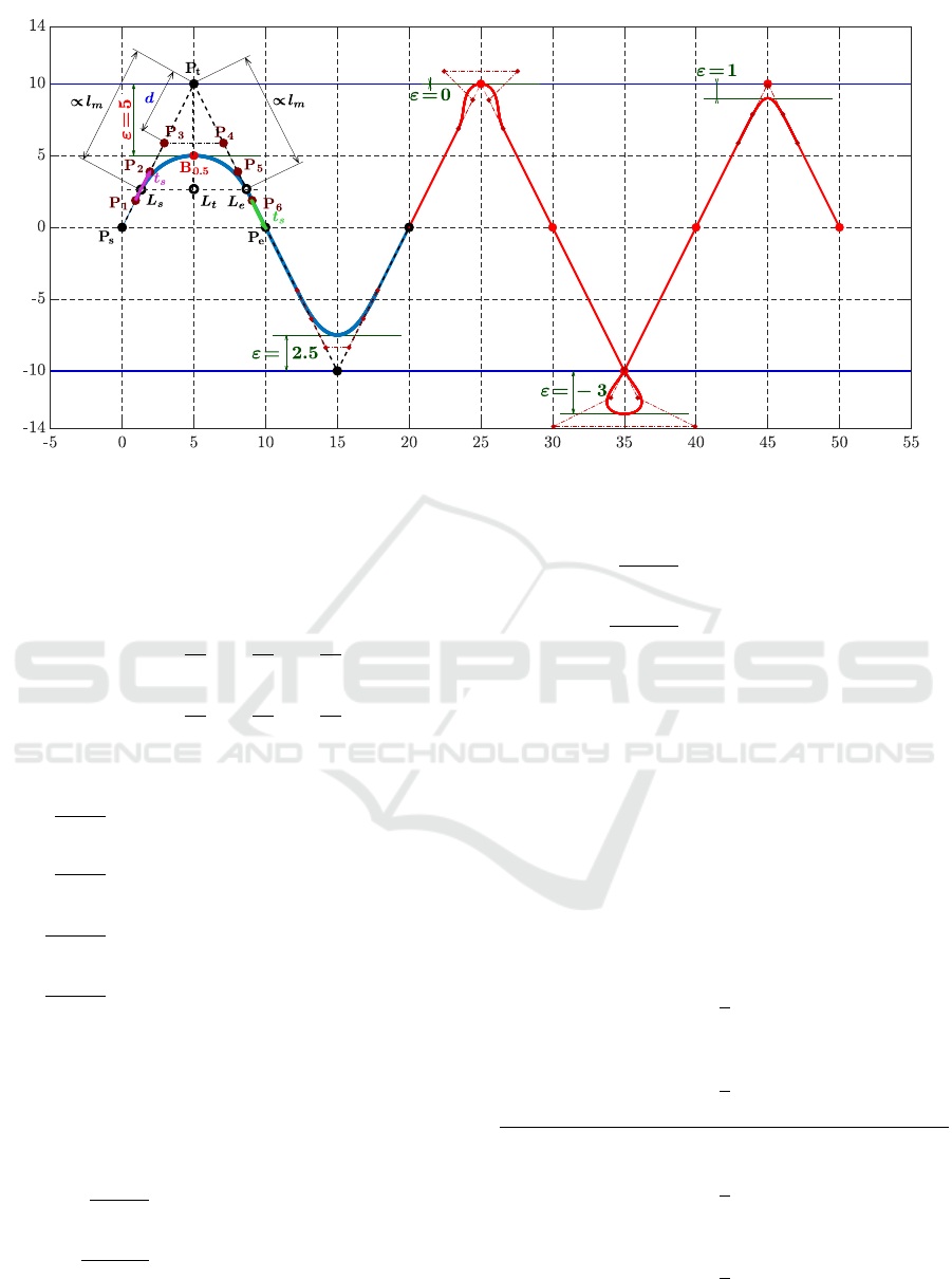
Figure 3: B
´
ezier parameters and examples of the smoothing for different required offsets (tolerances).
The explanation of individual parts is as follows:
i) evaluation of B
´
ezier points and derivatives
for u = 0, u = 0.5 and u = 1:
B(u)|
u=0
= P
1
(6)
B(u)|
u=0.5
=
1
32
P
1
+
5
32
P
2
+
10
32
P
3
+
10
32
P
4
+
5
32
P
5
+
1
32
P
6
(7)
B(u)|
u=1
= P
6
(8)
dB(u)
du




u=0
= 5(P
2
− P
1
) (9)
dB(u)
du




u=1
= 5(P
6
− P
5
) (10)
d
2
B(u)
du
2




u=0
= 20(P
3
− 2P
2
+ P
1
) (11)
d
2
B(u)
du
2




u=1
= 20(P
6
− 2P
5
+ P
4
) (12)
ii) points and derivatives for intersecting lines:
The initial description, used in this part, follows
from parametric equations of lines, see (13) and (16)
and Fig. 3:
L
s
(p) = P
s
+ p(P
t
− P
s
) (13)
dL
s
(p)
d p
= P
t
− P
s
(14)
d
2
L
s
(p)
d p
2
= 0 (15)
L
e
(p) = P
t
+ p(P
e
− P
t
) (16)
dL
e
(p)
d p
= P
e
− P
t
(17)
d
2
L
e
(p)
d p
2
= 0 (18)
Note that the parameter p, appearing in (13)
and (16), is a natural geometric parameter corre-
sponding to arc length of the segment. This parameter
will be used as the reference parameter in time param-
eterisations. Since the parameter of B
´
ezier curve u is
not linearly related to the arc-length, it will be also
transformed to the mentioned parameter p. However,
both parameters are considered as uniform parame-
ters, i.e. p ∈ h0, 1i as well as u ∈ h0, 1i by definition;
iii) comparison of corresponding derivatives
(for smooth joining of abscissas and B
´
ezier curve):
1
st
derivative: 5(P
2
− P
1
) = P
t
− P
s
(19)
⇒ P
2
=
1
5
(P
t
− P
s
) + P
1
(20)
2
nd
derivative: P
3
− 2P
2
+ P
1
= 0 (21)
⇒ P
3
=
2
5
(P
t
− P
s
) + P
1
(22)
1
st
derivative: 5(P
6
− P
5
) = P
e
− P
t
(23)
⇒ P
5
=
1
5
(P
t
− P
e
) + P
6
(24)
2
nd
derivative: P
6
− 2P
5
+ P
4
= 0 (25)
⇒ P
3
=
2
5
(P
t
− P
e
) + P
6
(26)
ICINCO 2019 - 16th International Conference on Informatics in Control, Automation and Robotics
232

iv) determining point B(u)|
u=0.5
:
l
s
=
p
(x
t
− x
s
)
2
+ (y
t
− y
s
)
2
+ (z
t
− z
s
)
2
l
e
=
p
(x
t
− x
e
)
2
+ (y
t
− y
e
)
2
+ (z
t
− z
e
)
2



l
m
= min(l
s
, l
e
) (27)
L
s
= P
t
+ (P
s
− P
t
)
(0.5l
m
)
l
s
L
e
= P
t
+ (P
e
− P
t
)
(0.5l
m
)
l
e



L
t
=
1
2
(L
s
+ L
e
) (28)
l
t
=
q
(x
L
t
− x
P
t
)
2
+ (y
L
t
− y
P
t
)
2
+ (z
L
t
− z
P
t
)
2
(29)
B(0.5) = P
t
+ ε
L
t
− P
t
l
t
(30)
v) expressing control points via parameter d:
Unknown control points of B
´
ezier curve can be ex-
pressed straightforwardly by specific distance d from
transition point (intersection point of two contiguous
lines). Specifically, d is the distance from transition
point P
t
to control points P
3
and P
4
.
t
s
=
P
t
− P
s
l
s
, (l
s
= kt
s
k) (31)
t
e
=
P
t
− P
e
l
e
, (l
e
= kt
e
k) (32)
P
1
= P
t
−
2
5
l
m
t
s
− d t
s
(33)
P
2
= P
t
−
1
5
l
m
t
s
− d t
s
(34)
P
3
= P
t
− d t
s
(35)
P
4
= P
t
− d t
e
(36)
P
5
= P
t
−
1
5
l
m
t
e
− d t
e
(37)
P
6
= P
t
−
2
5
l
m
t
e
− d t
e
(38)
vi) computation of the parameter d:
The computation of the searched parameter d is deter-
mined by eqs. (30) and (7) with eqs. (33) – (38).
B(0.5) = P
t
+ ε
L
t
− P
t
l
t

32B(0.5) = P
1
+ 5P
2
+ 10P
3
+ 10P
4
+ 5P
5
+ P
6
= 32P
t
− 16 d(t
s
+t
e
) −
7
5
l
m
(t
s
+t
e
)



⇒ d = 2
(P
t
− B(0.5))
.(t
s
+t
e
)
−
7
80
l
m
(39)
4 TIME PARAMETRIZATION
The time parametrization with respect to arc length
includes just computation of path length, time
parametrization with respect to arc length (timing
of geometric parameter p(t)) and decomposition
to the individual curve coordinates. The following in-
dividual sections will show related theoretical back-
ground.
4.1 Computation of the Path Length
Computation of the path length is defined as:
` = s(u)|
u=1
=
u=1
Z
0
ds =
u=1
Z
0
p
˙x
2
+ ˙y
2
+ ˙z
2
du (40)
The integral (40) can be evaluated analytically
only for simple segments such as lines or arcs. How-
ever, for B
´
ezier curve it is necessary to use some ap-
proximative numerical method. Here, it is suitable
to consider Simpson’s rule: The given interval of pa-
rameter u is divided into an even number of subin-
tervals by equidistant points, similarly as in the case
of the trapezoidal rule, and in any interval [u
2i
,u
2i+2
],
i = 0, 1,·· · ,
m
2
− 1, of the length 2h and the Newton-
Cotes formula is used, then the resulting formula is
b
Z
a
f (u)du =
1
3
h[ f (u
0
) + 4 f (u
1
) + 2 f (u
2
)
+ 4 f (u
3
) + ··· + 4 f (u
m−3
)
+ 2 f (u
m−2
) + 4 f (u
m−1
) + f (u
m
)] + E( f (u)) (41)
where f (u) =
p
˙x(u)
2
+ ˙y(u)
2
+ ˙z(u)
2
, h =
b−a
m
,
a = 0 and b = 1; and E( f (u)) = −
1
180
h
4
d
4
f
du
4
(o)
is a numerical error (Rektorys, 1994).
4.2 Timing of Geometric Parameter
Time parametrization based on arc length can be re-
alized according to selection of acceleration polyno-
mial a of 1
st
, 3
rd
or 5
th
order. For purpose of this
paper, let us consider acceleration polynomial a of 1
st
order. Other possibilities are described e.g. in (Heng
and Erkorkmaz, 2010; Huang and Zhu, 2016).
For the selection of the acceleration polynomial
of a of 1
st
order, there exist two main acceleration
shapes: triangular and trapezoidal, both with three
special cases: limit case without involved central zero
acceleration determining constant feed rate; start-up
and stop phases. The mentioned two main shapes are
illustrated in Fig. 4 (Belda and Novotn
´
y, 2012).
Smoothing and Time Parametrization of Motion Trajectories for Industrial Machining and Motion Control
233

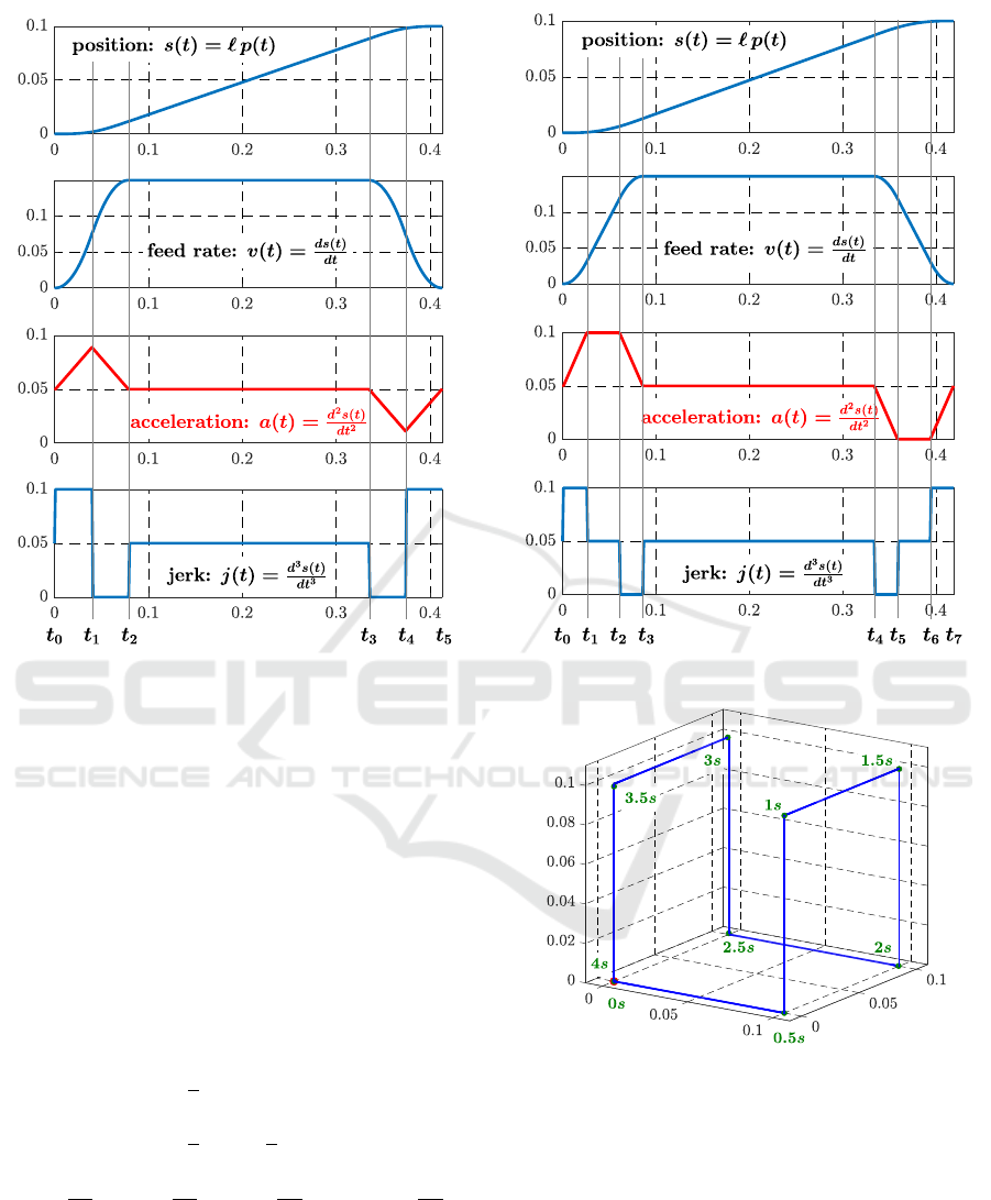
Figure 4: Kinematic quantities considering acceleration a(t) of 1
st
order with triangular (left) or trapezoidal (right) profile.
Time parametrization follows from the profiles
(Fig. 4) and it is determined for all indicated time in-
tervals, in which all related limiting kinematic quan-
tities ( j
max
, a
max
, v
max
) are considered. The intervals
for triangular acceleration profile are:
(t
0
, t
1
i, (t
1
, t
2
i, (t
2
, t
3
i, (t
3
, t
4
i and (t
4
, t
5
i;
and for trapezoidal acceleration profile are:
(t
0
, t
1
i, (t
1
, t
2
i, (t
2
, t
3
i, (t
3
, t
4
i, (t
4
, t
5
i, (t
5
, t
6
i and (t
6
, t
7
i.
In general, the following consecutive integration
is solved just within defined time intervals:
j(t) = a
0
, a
0
= k j
max
, k ∈ {−1, 0, 1} (42)
a(t) =
Z
j(t)dt = a
0
t + a
1
(43)
v(t) =
Z
a(t)dt =
1
2
a
0
t
2
+ a
1
t + a
2
(44)
s(t) =
Z
v(t)dt =
1
6
a
0
t
3
+
1
2
a
1
t
2
+ a
2
t + a
3
(45)
p(t) =
s(t)
`
, ˙p(t) =
v(t)
`
, ¨p(t) =
a(t)
`
and
...
p
(t) =
j(t)
`
.
The result of the integration are coefficients in indi-
vidual resulting equations. Then, the geometric pa-
rameter including its appropriate derivatives can be
applied in the decomposition of the motion trajectory
to individual coordinate components (axes) (Belda
et al., 2007).
Figure 5: Testing trajectory (axes in [m]).
5 REPRESENTATIVE EXAMPLES
5.1 Runs with Tolerances ≈ 10
−6
m
As was mentioned, the G-Code, used for comparative
runs, is already introduced in the Table 1. Its graph-
ical representation is in Fig. 5. The time labels show
approximative time and direction of the motion.
The used parameters of the runs is in the Table 2.
ICINCO 2019 - 16th International Conference on Informatics in Control, Automation and Robotics
234

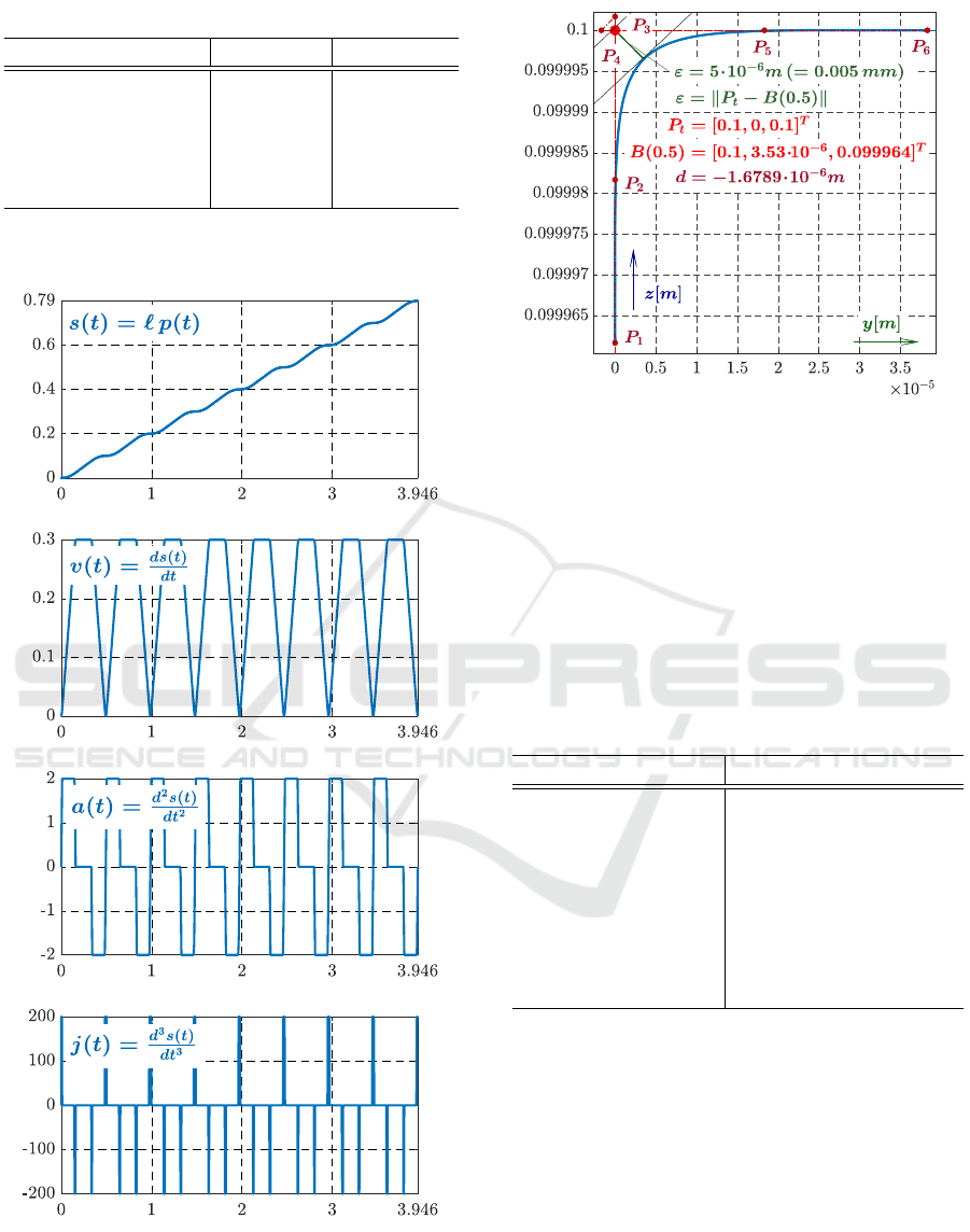
Table 2: Testing parameters.
parameter symbol value
admissible tolerance ε 5 · 10
−6
m
max. feed rate v
max
0.3ms
−1
max. acceleration a
max
2ms
−2
max. jerk j
max
200ms
−3
sampling period T
s
10
−3
s
The runs are shown in the following Fig. 6 -Fig. 7.
Figure 6: Time behaviours [s]: s(t), v(t), a(t), j(t).
Fig. 6 shows results of proposed smoothing algo-
rithm with time parametrization. Since the tolerance
ε = 0.005mm is too small, it is necessary to explore
Figure 7: Detail of smoothing with proposed algorithm.
the details in Fig. 7, which shows one B
´
ezier segment
of the testing geometric path (segment at front upper-
right vertex P
t
= [0.1, 0, 0.1]
T
). Total length saving is
0.04mm per 7 corners only. However, in sum in in-
dustrial machining, the saving is noticeable.
5.2 Example with Tolerances ≈ 10
−3
m
Values of d-parameter for set of B
´
ezier curves in gen-
eral 3D position (Fig. 8) are in the Table 3.
Table 3: List of d-parameters.
tolerance ε parameter d
ε
1
= 2.0 mm d
1
= 1.9223 mm
ε
2
= 1.5 mm d
2
= 1.2579 mm
ε
3
= 0.0 mm d
3
= −0.8750 mm
ε
4
= 1.0 mm d
4
= 0.3972 mm
ε
5
= −2.0 mm d
5
= −3.8915 mm
ε
6
= 3.0 mm d
6
= 3.5864 mm
ε
7
= −3.0 mm d
7
= −4.6811 mm
ε
8
= 0.5 mm d
8
= −0.2406 mm
6 CONCLUSION
This paper discusses the problem of smoothing con-
nection of linear segments by B
´
ezier curves. The re-
sults demonstrate achieving of prescribed tolerances
in the context of machine tools (≈ 10
−6
m) as well
as bigger motion (≈ 10
−3
m) for robotic case by de-
rived algorithm using MATLAB environment. Future
work will be focussed on on-line solution of smooth-
ing and time parametrization that will be able to con-
sider higher order polynomials.
Smoothing and Time Parametrization of Motion Trajectories for Industrial Machining and Motion Control
235

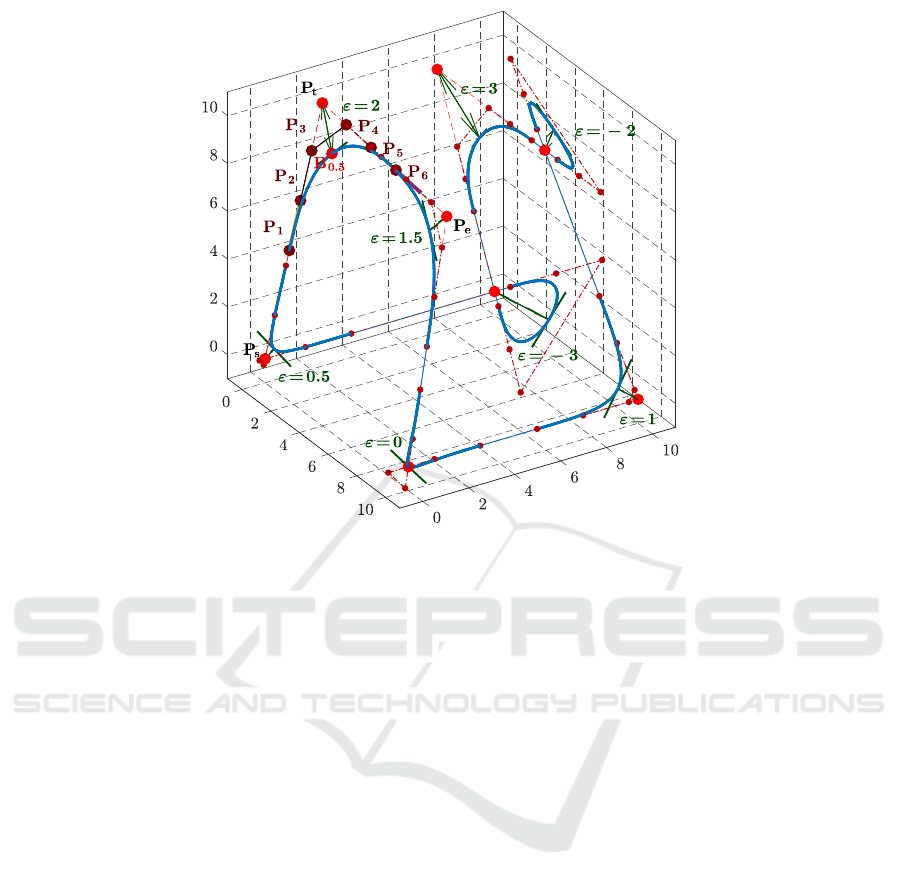
Figure 8: Example of general trajectory smoothing with tolerances ≈ 10
−3
m.
REFERENCES
Belda, K., B
¨
ohm, J., and P
´
ı
ˇ
sa, P. (2007). Concepts of
model-based control and trajectory planning for par-
allel robots. In Klaus, S., editor, Proc of 13th IASTED
Int. Conf. on Robotics and Applications, pages 15–20.
Acta Press.
Belda, K. and Novotn
´
y, P. (2012). Path simulator for ma-
chine tools and robots. In Proc. of the 17th Int. Conf.
on Methods and Models in Automation and Robotics,
pages 373–378. West Pomeranian University of Tech-
nology.
Erkorkmaz, K., Chen, Q.-G., Zhao, M.-Y., Beudaert, X.,
and Gao, X.-S. (2017). Linear programming and win-
dowing based feedrate optimization for spline tool-
paths. CIRP Annals, 66(1):393 – 396.
Heng, M. and Erkorkmaz, K. (2010). Design of a NURBS
interpolator with minimal feed fluctuation and contin-
uous feed modulation capability. Int. J. Machine Tools
& Manufacture, 50:281–293.
Huang, J. and Zhu, L. (2016). Feedrate scheduling for in-
terpolation of parametric tool path using the sine se-
ries representation of jerk profile. Proc. of the Inst.
of Mech. Engineers, Part B: J. Engineering Manufac-
ture, 231.
Luo, F.-Y., Zhou, Y.-F., and Yin, J. (2007). A universal
velocity profile generation approach for high-speed
machining of small line segments with look-ahead.
The Int. J. of Advanced Manufacturing Technology,
35(5):505–518.
Msaddek, E. B., Bouaziz, Z., Baili, M., and Dessein, G.
(2014). Influence of interpolation type in high-speed
machining (hsm). The Int. J. of Advanced Manufac-
turing Technology, 72(1):289–302.
Othman, A., Belda, K., and Burget, P. (2015). Physical
modelling of energy consumption of industrial articu-
lated robots. In Proc. 15th Int. Conf. on Control, Au-
tomation and Systems, ICCAS 2015, pages 784–789.
Institute of Control, Robotics and Systems, ICROS.
Piegl, L. and Tiller, W. (1997). The NURBS Book. Springer.
Rektorys, K. (1994). Survey of Applicable Mathematics.
Springer.
Sencer, B., Ishizaki, K., and Shamoto, E. (2015). A cur-
vature optimal sharp corner smoothing algorithm for
high-speed feed motion generation of NC systems
along linear tool paths. Int. J. Adv. Manuf. Technol.,
76:1977–1992.
Siemens (2019). NX docomentation. online.
Xavier, P., Yann, L., and Walter, R. (2010). Kinematic mod-
elling of a 3-axis NC machine tool in linear and circu-
lar interpolation. CoRR, pages 1004–2354.
Zhang, Y., , Zhao, M., Peiqing, Y., , Jiang, J., and Zhang,
H. (2018). Optimal curvature-smooth transition and
efficient feedrate optimization method with axis kine-
matic limitations for linear toolpath. The Int. J. of Ad-
vanced Manufacturing Technology, 99(1):169–179.
ICINCO 2019 - 16th International Conference on Informatics in Control, Automation and Robotics
236