Automatic Algorithmic Complexity Determination Using Dynamic
Program Analysis
Istvan Gergely Czibula, Zsuzsanna Onet¸-Marian and Robert-Francisc Vida
Department of Computer Science, Babes¸-Bolyai University, M. Kogalniceanu Street, Cluj-Napoca, Romania
Keywords:
Algorithmic Complexity, Dynamic Program Analysis.
Abstract:
Algorithm complexity is an important concept in computer science concerned with the efficiency of algo-
rithms. Understanding and improving the performance of a software system is a major concern through the
lifetime of the system especially in the maintenance and evolution phase of any software. Identifying certain
performance related issues before they actually affect the deployed system is desirable and possible if devel-
opers know the algorithmic complexity of the methods from the software system. In many software projects,
information related to algorithmic complexity is missing, thus it is hard for a developer to reason about the
performance of the system for different input data sizes. The goal of this paper is to propose a novel method
for automatically determining algorithmic complexity based on runtime measurements. We evaluate the pro-
posed approach on synthetic data and actual runtime measurements of several algorithms in order to assess its
potential and weaknesses.
1 INTRODUCTION
The performance of a software application is one of
the most important aspect for any real life software.
After the functional requirements are satisfied, soft-
ware developers try to predict and improve the per-
formance of the software in order to meet user expec-
tations. Performance related activities include modi-
fication of the software in order to reduce the amount
of internal storage used by the application, increase
the execution speed by replacing algorithms or com-
ponents and improve the system reliability and robust-
ness (Chapin et al., 2001).
Simulation, profiling and measurements are per-
formed in order to assess the performance of the sys-
tem during maintenance (McCall et al., 1985), but us-
ing just measurements performed on a developer ma-
chine can be misleading and may not provide suffi-
cient insight into the performance of the deployed sys-
tem on possible different real life data load. Profiling
is a valuable tool but, as argued in (W. Kernighan and
J. Van Wyk, 1998), no benchmark result should ever
be taken at face value.
Analysis of an algorithm, introduced by (Knuth,
1998) is concerned with the study of the efficiency of
algorithms. Using algorithm analysis one can com-
pare several algorithms for the same problem, based
on the efficiency profile of each algorithm or can rea-
son about the performance characteristics of a given
algorithm for increasing size of the input data. In
essence, studying efficiency means to predict the re-
sources needed for executing a given algorithm for
various inputs.
1.1 Motivation
While in case of library functions, especially stan-
dard library functions, complexity guarantees for the
exposed methods exist, such information is generally
omitted from the developer code and documentation.
The main reason for this is the difficulty of deduc-
ing said information by the software developer. Ana-
lyzing even a simple algorithm may require a good
understanding of combinatorics, probability theory
and algebraic dexterity (Cormen et al., 2001). Au-
tomated tools, created based on the theoretical model
presented in this paper can overcome this difficulty.
Knowledge about algorithmic complexity can
complement existing software engineering practices
for evaluating and improving the efficiency of a soft-
ware system. The main advantage of knowing the
complexity of a method is that it gives an insight into
the performance of an operation for large input data
sizes. Profiling and other measurement based tech-
niques can not predict the performance characteristics
of a method for other than the data load under which
186
Czibula, I., One¸t-Marian, Z. and Vida, R.
Automatic Algorithmic Complexity Determination Using Dynamic Program Analysis.
DOI: 10.5220/0007831801860193
In Proceedings of the 14th International Conference on Software Technologies (ICSOFT 2019), pages 186-193
ISBN: 978-989-758-379-7
Copyright
c
 2019 by SCITEPRESS – Science and Technology Publications, Lda. All rights reserved

the measurements were performed.
Knowledge about algorithmic complexity is also
beneficial for mitigating security issues in software
systems. There is a well documented class of low-
bandwidth denial of service (DoS) attacks in the lit-
erature that exploit algorithmic deficiencies in soft-
ware systems (Crosby and Wallach, 2003). The first
line of defence against such attacks would be to prop-
erly identify algorithmic complexity for the opera-
tions within the software system.
The main contributions of this paper is to pro-
pose and experimentally evaluate a deterministic ap-
proach to find the asymptotic algorithmic complexity
for a method. To the best of our knowledge there is
no other approach in the literature that automatically
determines algorithmic method complexity based on
runtime data analysis.
2 RELATED WORK
In this section we will present a short overview of
some existing approaches from the literature related
to algorithmic complexity.
The first approaches, for example (Le M
´
etayer,
1988), (Wegbreit, 1975) and (Rosendahl, 1989), were
based on source code analysis and the computation of
mathematical expressions describing the exact num-
ber of steps performed by the algorithm. While such
methods can compute the exact complexity bound of
an algorithm, they were defined for functional pro-
gramming languages and recursive functions.
More recent approaches can be applied for other
programming languages as well, but many of them
focus only on determining the complexity of spe-
cific parts of the source code (usually loops). Such
approach is the hybrid (composed of static and
dynamic analysis) method presented in (Demonti
ˆ
e
et al., 2015) and the modular approach presented in
(Brockschmidt et al., 2014).
Goldsmith et al. introduced in (Goldsmith et al.,
2007) a model that explains the performance of a pro-
gram as a feature of the input data. The focus is on
presenting the performance profile (empirical compu-
tational complexity) of the entire program and not the
identification of algorithmic complexity at the method
level.
Benchmark is a library, written in C++, that sup-
ports benchmarking C++ code (Benchmark, 2016).
Though it is not its main functionality, it also sup-
ports the empirical computation of asymptotic com-
plexities. A comparison of our approach to the results
provided by Benchmark are presented in Section 5.
While they do not focus on determining the com-
plexity of the source code directly, there are several
approaches that try to find performance bugs (pieces
of code that function correctly, but where functional-
ity preserving changes can lead to substantial perfor-
mance improvement) in the source code, for example:
(Luo et al., 2017), (Olivo et al., 2015) and (Chen et al.,
2018).
An approach using evolutionary search techniques
for generating input data that trigger worst case com-
plexity is presented in (Crosby and Wallach, 2003).
Such approaches are complementary to our approach
which assumes that testing data already exists.
3 METHODOLOGY
The most used representation for algorithm ana-lysis
is the one proposed in (Knuth, 1998), the asymptotic
representation, based on the Big O notation, a conve-
nient way to deal with approximations introduced by
Paul Bachmann in (Bachmann, 1894).
Definition 1. O( f (n)) denotes the set of g(n) such
that there exist positive constants C and n
O
with
|g(n)| ≤C ∗ f (n) for all n ≥n
0
.
If we denote by T (n) the number of steps per-
formed by a given algorithm (n is the size of the input
data), then the problem of identifying the algorithmic
complexity becomes finding a function f (n) such that
T (n) ∈ O( f (n)). The basic idea is to find a function
f (n) that provides an asymptotic upper bound for the
number of steps that is performed by the algorithm.
When analyzing algorithmic complexity, we are
not differentiating between functions like f (n) =
2n
2
+ 7 and f (n) = 8n
2
+ 2n + 1 the complexity in
both cases will be T (n) ∈ O(n
2
). The result of algo-
rithm analysis is an approximation indicating the or-
der of growth of the running time with respect to the
input data size (Cormen et al., 2001). While the com-
plexity function can be any function, there is a set of
well known and widely used functions in the literature
used to communicate complexity guarantees. In this
paper we use the functions from Table 1, but the set
can be extended without loosing the applicability of
the proposed method. The considered functions rep-
resent complexity classes that appear frequently for
real life software systems (Weiss, 2012).
In conclusion, the problem of identifying algorith-
mic complexity becomes selecting the most appropri-
ate function f (n) from a predefined set, such that f (n)
best describes the order of growth of the running time
of the analyzed method for increasing input data sizes.
In this paper we introduce an automated approach
for identifying algorithmic complexity for a method
Automatic Algorithmic Complexity Determination Using Dynamic Program Analysis
187

in a software system based on runtime measurements.
The basic idea is to measure the execution time of
the analyzed method for different input sizes and use
these measurements to identify the best fitting com-
plexity function. The proposed approach consists of
three steps described in the following sections.
3.1 Step 1 - Data Collection
Our approach requires multiple executions of the ana-
lyzed method with different input data and the record-
ing of the elapsed time for each execution. For this we
instrument the analyzed methods and implement code
that executes the target methods for different inputs.
Using Java profilers we were able to slightly modify
the entry and exit points of the targeted methods in
order to extract the information we needed, such as
execution time and input parameters. It is important
to note, that although these changes did impact the
execution a bit, they did not alter the original flow of
instructions in any way. This approach was chosen
since the profiler we used was not only lightweight,
adding little overhead to the original application, but
it was also highly reusable, being compatible with any
method we needed to analyze.
The result of the measurement step for a given
method mtd in a software system is a list of pairs
M
mtd
= {(t
i
, n
i
)}
m
i=1
where m is the number of mea-
surements performed for the method mtd, n
i
is the
size of the input data for the i-th measurement and
t
i
measures the elapsed time for running the analyzed
method with an input data of size n
i
.
3.2 Step 2 - Data Fitting
Given a set of measurements M
mtd
= {(t
i
, n
i
)}
m
i=1
and
a function f (n) from Table 1, we want to identify the
best coefficients c
1
, c
2
, such that the function fits the
actual measured data.
For example, for f (n) = c
1
n ·log
2
(n) + c
2
we try
to find c
1
, c
2
such that t
i
≈c
1
n
i
·log
2
(n
i
)+c
2
for every
measurement pair. For this purpose we use the non-
linear least square data fitting method (Hansen et al.,
2012), where we need to solve:
minimize
c
1
,c
2
f (c
1
, c
2
) =
m
∑
i=1
(t
i
−(c
1
n
i
·log
2
(n
i
) + c
2
))
2
For determining the best values for the coefficients
c
1
and c
2
, we used the scipy.optimize library from
Python, more exactly the curve
fit function from this
library (Scipy, 2019). Implementations for the curve
fitting algorithm are available in Matlab and other
programming languages and libraries as well.
In the definition of the Big O notation, the only re-
quirement regarding the constant C is that it should be
positive, but no upper limit is set, since the inequal-
ity from the definition should be true for all values
of n ≥ n
0
. However, in our approach the value n
(i.e., the size of the input data) is finite, it has a max-
imum value, which means that the values of the con-
stants c
1
, c
2
should also be restricted. If we consider
the function f (n) = c
1
log
2
(n)+c
2
, and the maximum
value of n (the maximum input size in the set M
mtd
)
is 100000, log
2
(100000) is approximately 17. By al-
lowing the value of c
1
to be 17, we actually transform
the function into log
2
2
(n).
In order to avoid the problem presented above, we
introduce an algorithm to automatically identify the
upper bounds for the coefficients. We restrict the val-
ues of c
1
and c
2
to be in an interval [b
l
, b
u
]. The
value of the lower bound, b
l
, is set to 0.1 for ev-
ery function. The value of the upper bound, b
u
is
computed separately for every function f (n) from Ta-
ble 1 and for every set of measurements, M
mtd
. For
computing the bounds, we searched for the maximum
value of n in M
mtd
, denoted by n
max
. We also con-
sidered the functions from Table 1 with c
1
= 1 and
c
2
= 0, ordered increasingly by their value for n
max
.
For every function f (n), we considered the previous
function, f
prev
(n) (we added the constant function,
f (n) = 1 as well, to have a previous for every func-
tion). The value of the upper bound is computed as
b
u
= p ∗( f (n
max
) − f
prev
(n
max
)), where p is a value
between 0 and 1, denoting the percent of the differ-
ence we want to consider. In all our experiments pre-
sented below, the value of p = 0.05 was used. If the
value b
u
is less than 0.1 (the lower bound) we set b
u
to
be 0.2. Table 2 contains the bounds computed for the
functions from Table 1 for n
max
equal to 10
4
. Since
we did not present actual data sets yet, this value was
taken just to provide an example for the bounds. In
Table 2 only the upper bounds for the functions are
given.
3.3 Step 3 - Select the Best Matching
Complexity Function
For a set of measurements M
mtd
= {(t
i
, n
i
)}
m
i=1
, and
for every function from Table 1 we computed at Step
2 the parameters c
1
, c
2
such that they represent the
best fit for the given function.
The aim of this step is to choose one single func-
tion that is the most accurate description of the mea-
surement data and consequently identify the complex-
ity class that the analyzed method belongs to. In order
to determine the best matching function, we compute
the RMSE (root mean square error) for every function
ICSOFT 2019 - 14th International Conference on Software Technologies
188

Table 1: Complexity classes considered for the experimen-
tal evaluation.
Name Function Complexity
class
F1 c
1
·log
2
(log
2
(n)) + c
2
log
2
(log
2
(n))
F2 c
1
·
p
log
2
(n) + c
2
p
log
2
(n)
F3 c
1
·log
2
(n) + c
2
log
2
(n)
F4 c
1
·log
2
2
(n) + c
2
log
2
2
(n)
F5 c
1
·n + c
2
n
F6 c
1
·nlog
2
(n) + c
2
nlog
2
(n)
F7 c
1
·n
2
+ c
2
n
2
F8 c
1
·n
2
log
2
(n) + c
2
n
2
log
2
(n)
F9 c
1
·n
3
+ c
2
n
3
F10 c
1
·n
4
+ c
2
n
4
Table 2: Examples of bounds for a data set with the maxi-
mum input data size 10
4
.
Func. Upper Bound Func. Upper bound
F1 0.2 F6 6143.856
F2 0.132 F7 4.99 ·10
6
F3 0.478 F8 6.14 ·10
7
F4 8.164 F9 4.99 ·10
10
F5 491.172 F10 5 ·10
14
F from Table 1 considering the values for c
1
and c
2
from Step 2. We pick as the complexity class best de-
scribing our data, the function F with the minimum
RMSE.
4 COMPUTATIONAL
EXPERIMENTS
In order to assess the effectiveness of the proposed
approach, we will perform a series of experiments on
synthetic data and actual measurements for different
algorithms. The experiments were chosen based on
the literature review, existing approaches in the liter-
ature use similar test systems. In the first experiment
we exemplify the potential of our approach using syn-
thetic measurement data. The second experiment is
performed on a small code base with various sorting
methods. Similar experiments where performed in
the literature in (Wegbreit, 1975) in order to evaluate
the effectiveness of their proposed approaches. The
scope of the last experiment is to illustrate the poten-
tial of the proposed approach beyond identifying the
runtime complexity of a method.
Table 3: Hidden functions used to generate data sets.
Name Function f (n) Complexity
class
HF1 5n
2
+ 20 n
2
HF2 3n
2
+ 7n + 20 n
2
HF3 log
2
(n) + 7 log
2
(n)
HF4 log
2
(n) +
p
log
2
(n)+ log
2
(n)
log
2
(log
2
(n))
HF5 4log
2
2
(n)+ log
2
2
(n)
11log
2
(n) + 25
HF6 n
2
log
2
(n) + 12n
2
n
2
log
2
(n)
HF7 9n + 15
√
n + 7 n
HF8 25n
3
+ 2n
2
+ 500n + 4 n
3
HF9 n
2
+ 500nlog
2
(n) n
2
HF10 20nlog
2
(n) + 100n + 3 nlog
2
(n)
4.1 Synthetic Data
The aim of the first experiment is to illustrate the pro-
posed method, to verify its potential and evaluate pos-
sible limitations. We generate multiple sets of syn-
thetic measurement data based on different mathemat-
ical functions. The assumption is that the number of
steps performed by a given method can be described
with a function. The set of functions used for these
experiments and the complexity class they belong to
is presented in Table 3. We used 10 different func-
tions in order to simulate multiple possible running
scenarios. From now on we will call these functions
hidden functions, based on the idea that, while they
describe the number of steps performed by an algo-
rithm, in general, they are not known.
We generate a separate data set for every hidden
function. Each data set contains 50 pairs of values
[n, f (n)] where n is ranging from 100 to 10 million,
evenly distributed in the mentioned interval. Intu-
itively every function corresponds to a method in a
software system and every generated pair corresponds
to a measurement (execute the method and collect in-
put data and elapsed time).
Using the generated data, we try to predict the run-
time complexity of every method, the input data for
every experiment is one data set and the output is a
function representing the complexity of the associated
method.
The first step is to compute the coefficients for ev-
ery considered complexity class from Table 1 based
on the points generated for the hidden functions from
Table 3. For this we used the method described in
Section 3.2.
The next step is to compute the root mean squared
error (RMSE) between the data and every considered
complexity function.
Automatic Algorithmic Complexity Determination Using Dynamic Program Analysis
189

The last step is to select the complexity function
that best describes the analyzed data set, basically we
pick the one with the smallest RMSE.
We performed the experiment for every data set
and our approach is able to correctly identify the
complexity class for every considered hidden function
from Table 3.
4.2 Sorting Methods Case Studies
The aim of this case study is to classify algorithms
into different complexity classes based on measure-
ment data. We measured (using the methodology
from Section 3.1) the running time for various sort-
ing methods in order to automatically determine their
complexity. We choose this experiment as other ap-
proaches in the literature related to the topic of algo-
rithmic complexity use as a case study similar exam-
ples.
The analyzed project includes various sorting
methods: insertion sort, selection sort, merge sort,
quicksort, bubble sort, heapsort and code that exe-
cutes those methods for different lists of numbers.
4.2.1 Collecting Measurements
The code will invoke each sorting method for arrays
sorted in ascending order, descending order and with
elements in random order, varying the length of the
array for each invocation. We have chosen these types
of input array orderings, because, for many sorting
algorithms, they are connected to the best, worst and
average case runtime complexity of the algorithm.
We generated the input arrays of numbers in as-
cending, descending and random order. As presented
above we have considered 6 different sorting algo-
rithms, but for quicksort we considered two different
implementations: one in which the first element of
the arrays is always chosen as the pivot (this version
will be called quicksort first), and one where the mid-
dle element was always chosen as the pivot (quicksort
middle). The expected correct results for all sorting
algorithms and the 3 input array orderings are pre-
sented in Table 4, where asc. means ascending, desc.
means descending and rnd. means random.
We run the experiments on two regular laptops
with different hardware specifications. A first group
of data sets were created on one laptop, denoted by L
1
,
where for each of the above mentioned 7 sorting al-
gorithms (considering both versions of quicksort) and
for each of the three input array orderings (ascending,
descending and random) we have created four data
sets. This gives us a total of 84 L
1
data sets.
A second group of data sets were created on a sec-
ond laptop, denoted by L
2
, where for each of the sort-
Table 4: Correct complexity classes for the considered al-
gorithms and input array orderings.
Algorithm Asc. Desc. Rnd.
insertion sort n n
2
n
2
selection sort n
2
n
2
n
2
merge sort nlog
2
(n) nlog
2
(n) nlog
2
(n)
quicksort first n
2
n
2
nlog
2
(n)
quicksort mid. nlog
2
(n) nlog
2
(n) nlog
2
(n)
bubble sort n n
2
n
2
heapsort nlog
2
(n) nlog
2
(n) nlog
2
(n)
ing algorithms (for quicksort one single version was
considered, quicksort first) and for each of the input
array orderings, we have created one data set. This
gives us a total of 18 L
2
data sets.
In order to test the generality of our approach, we
have created data sets containing measurements for
C++ code as well. For these data sets, the measure-
ments were performed using the Benchmark library
(Benchmark, 2016). For each of the 7 sorting algo-
rithms, and for each of the three input array orderings
we have created two data sets, a short one and a long
one (the exact number of points is given below). For
this group, we have a total of 42 data sets and we call
it the BM data sets.
Each of the 144 data sets contains between 31 and
37 pairs of measurements representing the size of the
array and the run-time in nanoseconds. The set of 37
different array sizes is S = {s ∈ N|s = i ·10
j
, s <=
2 ·10
6
, i ∈ N ∩[1, 9], j ∈ N ∩[2, 6]}. The exact num-
ber of measurements for every sorting algorithm and
group is presented in Table 5. The data sets with less
than 37 points do not contain measurements for the
last points of the above list because running the corre-
sponding algorithms would have taken too much time
(for example, in case of bubble sort in group L
1
, the
last data point is for an array of length 500000).
Table 5: Number of measurements for data sets.
Group Sorting method Number of points
L
1
insertion sort 37
selection sort 37
merge sort 37
quicksort first 32
quicksort middle 32
bubble sort 32
heapsort 37
L
2
all data sets 36
BM
short data sets 31
long data sets 37
ICSOFT 2019 - 14th International Conference on Software Technologies
190

4.2.2 Determining the Complexity for Sorting
Data
We have performed an experiment similar to the one
presented in Section 4.1: for every data set we deter-
mined the complexity class which is the best match
for the points from the data set. We have considered
the 10 complexity classes from Table 1.
From the 144 data sets, our algorithm returned the
correct complexity class (i.e., the ones from Table 4)
for 137 data set, having an accuracy of 95%.
Considering these results we can conclude that our
approach can identify the complexity class based on
runtime measurement data with a good accuracy.
4.2.3 Data Set Size Reduction
The next step of this experiment is to verify if the ob-
tained accuracy is maintained even if we reduce the
number of recorded measurement samples. From ev-
ery data set we have randomly removed points: first
we removed one point randomly and run our approach
to determine the complexity class to which the re-
maining points belong. Then, starting from the orig-
inal data set, we removed two points and determined
the complexity class for the remaining points. And so
on, until only 5 points remained. We repeated each
experiment 100 times and counted how many times
the correct result was obtained, which is the accuracy
for the given data set.
For every sorting algorithm and input array order-
ing (ascending, descending, random), we computed
the average accuracy over the 7 data sets (6 in case
of quicksort middle) and two of these are presented in
Figure 1. The accuracy is computed for data sets with
the same number of points left.
Due to lack of space, Figure 1 does not contain all
sorting algorithms. We did not include the results for
quicksort middle, heap sort, selection sort and merge
sort because for these algorithms the accuracy is al-
most 100% for each case. We did not include bubble
sort either, which is similar to insertion sort.
The two sorting algorithms from Figure 1 contain
lower accuracy values for some array orderings. In
case of insertion sort, descending and random array
have almost perfect accuracy (above 98% for every
case), but for ascending arrays the accuracy is be-
tween 83% and 53%. The reason for these decreased
values is that for the two ascending BM data sets our
approach did not find the correct complexity class for
the initial data sets and it has an accuracy of 0 (for
these two data sets) when we start removing points.
Quicksort first is another sorting algorithm for
which our approach could not find the correct com-
plexity class in every case and this is visible on Figure
1 as well. For quicksort first, an incorrect result was
returned for the ascending and descending array from
the L
2
group, and for these two data sets the accuracy
is constantly 0 when we remove elements.
As expected, the quality and quantity of the mea-
surements influence the accuracy of our approach, but
the results are still promising and further work will be
done in order to identify bottlenecks.
4.3 Map Case Study
The aim of this case study is to show the potential of
the proposed approach to identify non-obvious perfor-
mance related problems in real life software systems.
The Map (Dictionary) is a widely used data type
described as an unsorted set of key-value elements
where the keys are unique. For this discussion we will
refer to the HashMap implementation available in the
Java programming language.
Given an implementation similar with the one
from Figure 2 an average software developer would
assume an algorithmic runtime complexity n for tar-
getMethod where n is the number of keys in the Map.
For most use cases this assumption is true. How-
ever, we managed to write specially crafted code for
which, based on runtime measurements, our approach
returned the complexity classes n
2
and nlog
2
n, which
are worse than developers’ intuition.
While the results may look surprising or erro-
neous, they are in fact correct. In order to get a com-
plexity class of n
2
, we need to make sure that every
key has the same hash code, so they will all be added
into the same bucket. In this way finding one key will
have a complexity of n.
The nlog
2
n complexity is obtained when the keys
are comparable, because in this situation in the Java
implementation of HashMap the individual buckets
will switch to a balanced tree representation when-
ever the amount of elements within exceeds a thresh-
old. Assuming that all elements have the same hash
code, searching for a key will have a complexity of
log
2
n. After a closer look into the HashMap docu-
mentation, specifically this change (OpenJDK, 2017),
we find out about this lesser known behaviour.
Our approach can be used to develop automated
tools that identify performance related problems and
to indicate possible security issues that can be ex-
ploited by malicious users or systems that try to ex-
ploit algorithmic deficiencies. While in this experi-
ment we created special code to reproduce the perfor-
mance issue, measurement data can be collected by
other means (Section 3.1).
Automatic Algorithmic Complexity Determination Using Dynamic Program Analysis
191

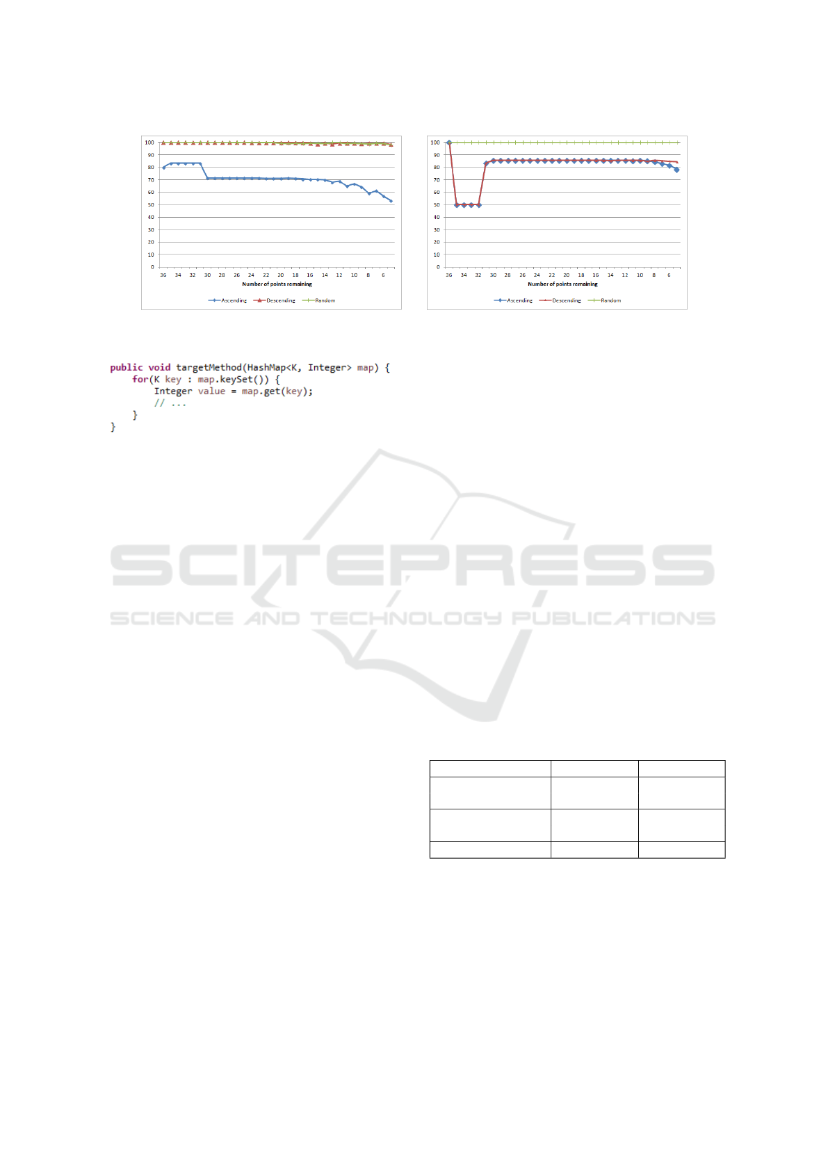
(a) Insertion sort (b) Quicksort first
Figure 1: Average accuracy over the sorting data sets after the removal of points.
Figure 2: HashMap data collection function.
5 DISCUSSION AND
COMPARISON TO RELATED
WORK
In Section 4.1 we illustrated experimentally that our
approach is able to correctly identify the runtime
complexity even from a small number of measure-
ment samples.
Input and output blocking instructions, network
communication as well as multithreaded operations
are not specifically handled with our approach, so at
first glance one might see this as a problem. However,
this is fine considering that our analysis would be per-
formed in a test, where one could mock blocking in-
structions. Furthermore, even if it was not possible to
eliminate these aspects from our analysis, we would
still want to be able to measure the performance of the
rest of the code.
The running time may not reflect the number of
steps performed by the algorithm. For practical rea-
sons the actual runtime is more important, and with
the aid of other tools such as profilers, we can identify
the factors that influenced said execution durations.
The most similar approach to the one proposed
in this paper is Benchmark (Benchmark, 2016), but
it can only be used for computing the complexity of
C++ code. However, since it is an open source library,
we implemented their method in Python to compare it
with our proposed approach. We have used two set-
tings for the experiments: one in which all the com-
plexity classes considered for our approach (the ones
from Table 1) were considered and one experiment in
which only those six complexity classes were consid-
ered, which are used in the Benchmark library as well
(this included the constant complexity class as well,
which is not used in our approach).
For the first setting, the Benchmark implementa-
tion found the correct complexity class for 55 out of
144 data set, an accuracy of 38%. For the second set-
ting, the results were better, 83 correctly classified
data sets, resulting in an accuracy of 58%. The ac-
curacy for our approach on these data sets, was 95%,
which is a lot better. Moreover, for the data set for
which our approach did not find the correct complex-
ity class, neither did the benchmark implementation.
However, Benchmark was developed for C++
code, so an explanation for the poor performance can
be the large number of data sets (102 out of 144) con-
taining measurements for Java code. In order to in-
vestigate this theory, we measured the accuracy sepa-
rately for the C++ data sets (generated using Bench-
mark) and the Java data sets. The accuracies are pre-
sented in Table 6.
Table 6: Accuracies for C++ and Java data sets for our ap-
proach and the Benckmark implementations.
Method C++ data set Java data set
Benchmark 10 76% 23 %
complexity classes
Benchmark 6 81 % 48%
complexity classes
Our approach 90% 97 %
From Table 6 we can see that considering only
the data sets generated for C++ code, the accuracy
of the Benchmark implementation is approximately
twice as high as for the Java data sets. This suggests
that determining the complexity class for Java code is
more complicated than determining it for C++ code
and more complex methods are needed for it.
Other approaches in the literature focus on a spe-
cific type of algorithms (such as (Zimmermann and
ICSOFT 2019 - 14th International Conference on Software Technologies
192

Zimmermann, 1989) dealing with divide and conquer
algorithms) or specific parts of the code (such as loops
in (Demonti
ˆ
e et al., 2015)). Our approach is more
general, it is not constrained by the type of algorithm
used in the analyzed method. We focus on an entire
method that has the additional benefit that the instru-
mented code used to collect runtime data is less costly
since our only concern is the execution time of the
method.
6 CONCLUSIONS AND FUTURE
WORK
In this paper we have introduced an approach for auto-
matically determining the algorithmic complexity of a
method from a software system, using runtime mea-
surements. The results of the experimental evaluation
show the potential of our approach. Although the ap-
proach has a good accuracy, further improvement is
possible by analyzing the particularities of the mis-
classified examples.
The next step would be automatizing this whole
process and making it readily available to developers.
The research and experiments described in this paper
serve as solid groundwork for creating such a tool that
allows for real time algorithm complexity verification.
The need for this functionality becomes clear when
one considers the benefits gained, such as the abil-
ity to easily identify potential performance or security
misconceptions developers might have when writing
the code. The exact manner in which said tool might
function still needs analysis and experimentation, but
a possible form might be akin to unit tests that are ex-
ecuted within a continuous integration environment.
REFERENCES
Bachmann, P. (1894). Die Analytische Zahlentheorie.
Benchmark (2016). Benchmark library.
https://github.com/google/benchmark.
Brockschmidt, M., Emmes, F., Falke, S., Fuhs, C., and
Giesl, J. (2014). Alternating runtime and size com-
plexity analysis of integer programs. In International
Conference on Tools and Algorithms for the Con-
struction and Analysis of Systems, pages 140–155.
Springer.
Chapin, N., Hale, J. E., Kham, K. M., Ramil, J. F., and Tan,
W.-G. (2001). Types of software evolution and soft-
ware maintenance. Journal of Software Maintenance,
13(1):3–30.
Chen, Z., Chen, B., Xiao, L., Wang, X., Chen, L., Liu, Y.,
and Xu, B. (2018). Speedoo: prioritizing performance
optimization opportunities. In 2018 IEEE/ACM 40th
International Conference on Software Engineering
(ICSE), pages 811–821. IEEE.
Cormen, T. H., Stein, C., Rivest, R. L., and Leiserson, C. E.
(2001). Introduction to Algorithms. McGraw-Hill
Higher Education, 2nd edition.
Crosby, S. A. and Wallach, D. S. (2003). Denial of ser-
vice via algorithmic complexity attacks. In Proceed-
ings of the 12th Conference on USENIX Security Sym-
posium - Volume 12, SSYM’03, pages 3–3, Berkeley,
CA, USA. USENIX Association.
Demonti
ˆ
e, F., Cezar, J., Bigonha, M., Campos, F., and
Magno Quint
˜
ao Pereira, F. (2015). Automatic infer-
ence of loop complexity through polynomial interpo-
lation. In Pardo, A. and Swierstra, S. D., editors, Pro-
gramming Languages, pages 1–15, Cham. Springer
International Publishing.
Goldsmith, S. F., Aiken, A. S., and Wilkerson, D. S. (2007).
Measuring empirical computational complexity. In
Proceedings of the the 6th Joint Meeting of the Euro-
pean Software Engineering Conference and the ACM
SIGSOFT Symposium on The Foundations of Software
Engineering, ESEC-FSE ’07, pages 395–404, New
York, NY, USA. ACM.
Hansen, P., Pereyra, V., and Scherer, G. (2012). Least
Squares Data Fitting with Applications. Least Squares
Data Fitting with Applications. Johns Hopkins Uni-
versity Press.
Knuth, D. E. (1998). The Art of Computer Programming,
Volume 3: (2Nd Ed.) Sorting and Searching. Addison
Wesley Longman Publishing Co., Inc., Redwood City,
CA, USA.
Le M
´
etayer, D. (1988). Ace: An automatic complexity eval-
uator. ACM Trans. Program. Lang. Syst., 10:248–266.
Luo, Q., Nair, A., Grechanik, M., and Poshyvanyk, D.
(2017). Forepost: Finding performance problems au-
tomatically with feedback-directed learning software
testing. Empirical Software Engineering, 22(1):6–56.
McCall, J. A., Herndon, M. A., Osborne, W. M., and States.,
U. (1985). Software maintenance management [mi-
croform] / James A. McCall and Mary A. Herndon,
Wilma M. Osborne. U.S. Dept. of Commerce, Na-
tional Bureau of Standards.
Olivo, O., Dillig, I., and Lin, C. (2015). Static detection of
asymptotic performance bugs in collection traversals.
In ACM SIGPLAN Notices, volume 50, pages 369–
378. ACM.
OpenJDK (2017). Hashmap implementation change.
https://openjdk.java.net/jeps/180.
Rosendahl, M. (1989). Automatic complexity analysis. In
Fpca, volume 89, pages 144–156. Citeseer.
Scipy (2019). Python scipy.optimize documentation.
https://docs.scipy.org/doc/scipy/reference/optimize.html.
W. Kernighan, B. and J. Van Wyk, C. (1998). Timing tri-
als, or, the trials of timing: Experiments with scripting
and user-interface languages. Software: Practice and
Experience, 28.
Wegbreit, B. (1975). Mechanical program analysis. Com-
munications of the ACM, 18(9):528–539.
Weiss, M. A. (2012). Data Structures and Algorithm Anal-
ysis in Java. Pearson Education, Inc.
Zimmermann, P. and Zimmermann, W. (1989). The auto-
matic complexity analysis of divide-and-conquer al-
gorithms. Research Report RR-1149, INRIA. Projet
EURECA.
Automatic Algorithmic Complexity Determination Using Dynamic Program Analysis
193