
Manifold Learning to Identify Consumer Profiles in Real Consumption
Data
Diego Perez
a
, Marta Rivera-Alba
b
and Alberto Sanchez-Carralero
c
Research, Clarity AI, New York, U.S.A.
Keywords:
Manifold Learning, Big Data, Consumer Data, Econometrics, Consumption Profiles.
Abstract:
Precise and comprehensive analysis of individual consumption is key to marketers and policy makers. Tra-
ditionally, people’s consumption profiles have been approximated by household surveys. Although insightful
and complete, household surveys suffer from some biases and inaccuracies. To compensate for some of those
biases, we propose a new approach to compute and analyze consumer profiles based on millions of purchase
transactions collected by a personal financial manager. Since this new kind of data sources requires new anal-
ysis methods, in this paper we propose the use of manifold learning techniques to visualize the whole data set
at once, demonstrating how these techniques can cluster consumers in more meaningful groups than demo-
graphics alone. These unsupervised behavior-based clusters allow us to draw more educated hypotheses that
we could otherwise miss. As an example, we will specifically discuss the characteristics of individuals with
high housing and recreation consumption in our sample.
1 INTRODUCTION
Understanding people’s priorities and desires has al-
ways been a challenge for marketers and policy mak-
ers. This knowledge guides marketers in their cam-
paigns and, perhaps more importantly, it guides policy
makers to come up with approaches catering to those
demographic groups more in need (Deaton, 2001;
Deaton et al., 1980). Because individuals rely on ex-
ternally supplied goods and services to satisfy their
needs, the analysis of consumption serves as rele-
vant approximation to people’s preferences and needs
(Deaton, 1997).
In order to estimate consumption data, researchers
have traditionally asked consumers directly through
household surveys (Deaton and Zaidi, 2002). These
surveys suffer from some biases, perhaps the most im-
portant one being the response bias—some groups are
more eager to respond than others—making parts of
the population invisible or underrepresented in house-
hold surveys (Groves, 2006; Christian, 2012; Furn-
ham, 1986). Moreover, these surveys focus on con-
sumption at the household level. Although this could
make sense for many analyses, it misses the individ-
a
https://orcid.org/0000-0002-1837-2270
b
https://orcid.org/0000-0002-8069-385X
c
https://orcid.org/0000-0002-1966-2800
ual preferences within the household. For example,
the behavior of non-emancipated young adults with
their own salary and expenses is diluted when aggre-
gating household consumption. Analyzing this popu-
lation segment is specially relevant when forecasting
future consumption trends.
An alternative to asking people directly about their
preferences through surveys is measuring their con-
sumption behavior. The global adoption of electronic
payment systems and mobile devices open new op-
portunities to collect behavioral data—after the nec-
essary anonymization protocols. Compared to house-
hold surveys, behavioral data shows increased indi-
vidual resolution, lower costs, and alternative pop-
ulation sampling–with complementary selection bi-
ases to surveys. In this paper we used a behavioral
data set collected from a Personal Financial Manager
in Spain. Our data set includes millions of transac-
tions from almost 50 thousand anonymous users. As
a comparison, the national Spanish consumption sur-
vey include less households for a larger cost (INE,
2017). From our transaction data set we computed the
complete consumer profiles in a given year. Although
anonymous, the data set includes some demographic
information about the users sampled, which allows us
to analyze the consumption patterns of thousands of
individuals with either individual or demographic res-
olutions.
Perez, D., Rivera-Alba, M. and Sanchez-Carralero, A.
Manifold Learning to Identify Consumer Profiles in Real Consumption Data.
DOI: 10.5220/0007832400230031
In Proceedings of the 8th International Conference on Data Science, Technology and Applications (DATA 2019), pages 23-31
ISBN: 978-989-758-377-3
Copyright
c
2019 by SCITEPRESS – Science and Technology Publications, Lda. All rights reserved
23

Addressing the visualization and analysis of these
new large data sets challenges traditional statisti-
cal tools. Over the recent years, several research
groups have developed new supervised and unsuper-
vised machine-learning techniques to analyze them
(Di Clemente et al., 2018; Pentland, 2013). In this pa-
per we use an unsupervised method known as t-SNE
(Maaten and Hinton, 2008). t-SNE is an non-linear
embedding technique based on manifold learning able
to represent all of our high dimensional consumer
profiles in a two dimensional space, while aiming
to keep the original relative distance between users.
This embedded representation can be used as a basis
for more relevant clustering than demographic seg-
ments. In addition, unsupervised methods like t-SNE
can produce more meaningful and sometimes counter
intuitive insights from the data set that could be other-
wise missed. As an example, in this paper we used the
t-SNE embedding to identify two clusters of individ-
uals: one with above average housing consumption,
and other with above average recreation consumption.
We found middle-age individuals over-indexing in the
former, and younger, poorer males over-indexing in
the latter.
The remainder of this paper is structured as fol-
lows: section 2 describes the methods, including a
data overview and description of consumption cat-
egories, section 3 describes the results of the pa-
per, section 3.1 outlines our pipeline for construct-
ing consumption profiles from micro-transaction data
and explore the mean consumer profile in our sample,
section 3.2 explores the differences in consumption
across demographics, section 3.3 shows the problems
of this traditional approach, section 3.4 shows how
manifold learning can serve as a basis for more rel-
evant clusters, allowing us to analyse independently
the consumers of specific categories, and finally we
discuss our results in section 4.
2 METHODS
2.1 Data Overview
The data set used is comprised of almost 24 million
banking transactions from 49965 users of a Spain-
based Personal Finance Management service. The
data set covers all transactions for those users in 2017
including inbound/outbound money transfers, card
payments and cash withdrawals. In this work we only
analyzed transactions that can be connected to a con-
sumption category (section 2.2 and Appendix). Each
user is described by its Region, Age range, Income
range, and Gender. Demographic slices are struc-
tured as follows:
• Region contains the Spanish region—Comunidad
Autonoma—where the user lives.
• Age range is divided in the following ranges: 18
to 25, 26 to 35, 36 to 45, 46 to 55 and Over 55.
• Income range encloses ranges divided by the an-
nualized average monthly income. The ranges
are the following: Under e584, e584 to e1,083,
e1,084 to e1,583, e1,584 to e2,416, e2,417 to
e3,333, e3,334 to e4,166, e4,167 to e5,000,
e5,001 to e5,834 and Over e5,834
• Gender: Male or female.
Since the main objective of this paper is not to an-
alyze the Spanish population, but to introduce novel
methods to analyze big data sources, data is not re-
sampled to mimic the Spanish population—as ex-
plained in the next sections this reduces the complex-
ity of the approach. The full description of the sample
distribution across regions, age ranges, income ranges
and gender can be found at Appendix. Significance
is measured based on data sample. Users have given
express consent to research and commercial exploita-
tion of the data, in accordance with GDPR—General
Data Protection Regulation—(Council of European
Union, 2016) regulations. Data has been irreversibly
anonymized using differential privacy techniques.
2.2 Consumption Categories
We used our proprietary classification on consump-
tion categories based on the COICOP standard (Clas-
sification of Individual Consumption according to
Purpose) for households developed by the United
Nations Statistics Division (United Nations, DESA,
2018). This standard classifies consumption based on
the purpose of goods or services acquired. Our orig-
inal proprietary classification includes 42 categories,
but the granularity of this data set allows us to map
our transactions to 27 of them (Appendix). Although
all calculations in this work include all 27 categories,
in the interest of clarity, most of the graphics on this
paper include only the 12 most relevant categories.
Transactions in the categories of loans and trans-
fers are reassigned to category Housing based on
amount, recurrence, and whether the corresponding
user has been identified as a loan or mortgage owner.
Transactions in low-frequency categories at the com-
merce level —those covering less than 4% of the
total—, were reassigned at random, keeping the rela-
tive proportions of the rest of categories for that com-
merce.
DATA 2019 - 8th International Conference on Data Science, Technology and Applications
24
3 RESULTS
3.1 Consumption Profiles
Understanding people’s consumption profiles re-
quires a individual representation of that consump-
tion. To generate that representation we aggregated
the full list of annual transactions for each user in
27 different consumption categories (see section 2.2).
We then defined the consumption vector of a given
user as a 27-dimensional vector including the relative
spent of each category.
Consumption vectors can be aggregated to obtain
the mean consumption vector of the total data set (Fig.
1), or subsets of the sample, as we will see in the next
sections. These aggregated consumption vectors al-
low us to analyze general consumption trends in our
sample and could allow other researchers to find in-
sights on global patterns.
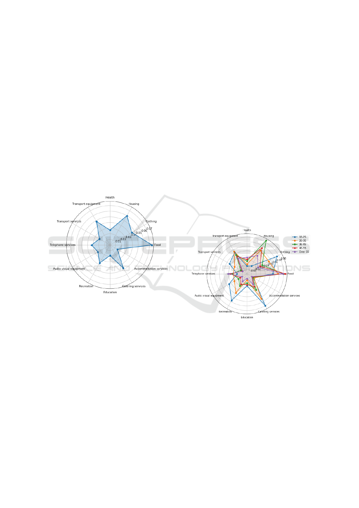
Figure 1: Average relative consumption on principal cate-
gories. Each point represents the mean relative spent in each
selected category for the total data set.
Among the 12 selected categories, we observed
the highest relative spent on Food, Housing, Trans-
port equipment and Catering services. In addition,
we also observed some particularities of the Spanish
population: for example, we found low spending on
Health and Education, as they are largely covered by
the public system (OECD/European Observatory on
Health Systems and Policies, 2017; Rogero-Garc
´
ıa
and Andr
´
es-Candelas, 2014).
Although averaging consumption vectors across
our entire sample gave us an idea about general pat-
terns of behavior, it lacks granularity. For example,
as we explored in the next sections, it is not feasible
to compare more than one demographic slice of the
sample at the same time.
3.2 Demographic Slices
Besides identifying global patterns, consumption pro-
file analysis is able to explore more granular and spe-
cific insights for target demographic slices. Splitting
the population in different groups allow us to analyze
different consumption profiles and study differences
and similarities between them.
Many studies have split the population by demo-
graphic profiles (Behrendt, 2005; Morris et al., 2006).
By way of illustration, we compare the mean con-
sumption vector across age ranges in Fig. 2. Re-
flecting peculiarities of the Spanish population, these
age-based mean spending vectors vary widely across
age ranges: for example, the oldest range spends rela-
tively more than the rest on Health, and the youngest
range spends relatively more than other slices on
Clothing, Transport, and Recreation. This represen-
tation already suggests that younger population is less
likely to spend in Housing than middle-age ranges, as
we will explore deeper in future sections. In addi-
tion, the data also suggests that the younger you are,
the more you spend in Recreation and Transport Ser-
vices.
Figure 2: Average consumption profile by age range. Each
line represents the mean consumption vector of the specific
age range.
Radar charts (Fig. 1 and Fig. 2) are a clear and
straightforward approach to represent consumption
vectors. Nevertheless, they can become complicated
to understand when comparing several demographic
dimensions at once. In those cases, we could use
pyramid plots. As an illustration, we split our sample
by age and gender in order to analyze the relative con-
sumption on Recreation. We observed that younger
users are the ones spending more in that category and
male users spend relatively more than females (Fig.
3).
A pyramid plot (Fig. 3) allowed us to add another
demographic dimension. However, it is still unable to
Manifold Learning to Identify Consumer Profiles in Real Consumption Data
25
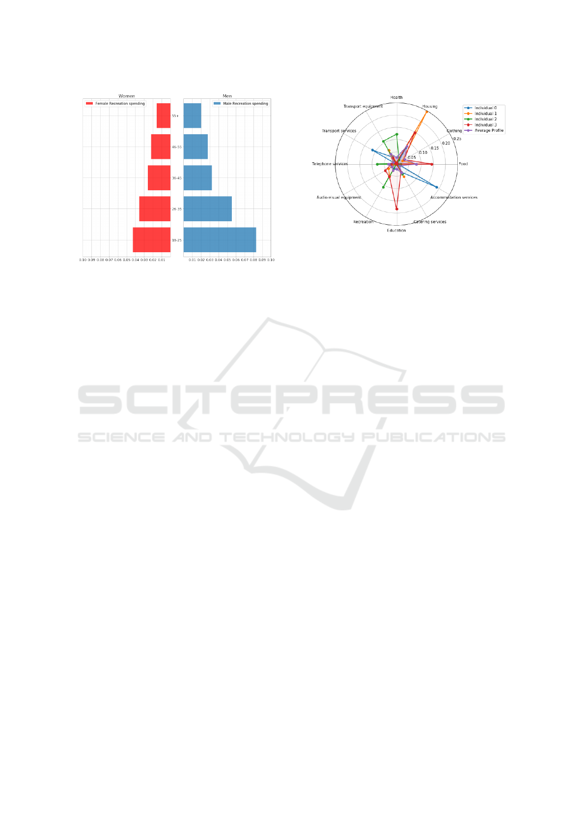
Figure 3: Recreation budget share by age and gender. On
the left (red): females and on the right (blue): males. Age
ranges are ordered as vertical axis.
represent more than two slices of the sample or show-
ing different consumption categories at a time. As a
solution, we could stack those categories in the same
plot, but generated plots could be difficult to interpret.
3.3 Problems of Demographic Slices
When splitting the population by demographic slices,
we implicitly assume that those slices are meaningful
for our analysis. In this section, we explore the valid-
ity of this hypothesis by measuring the behavioral ho-
mogeneity within each slice. We find evidence to the
contrary in the form of consumption profiles hetero-
geneity even when restricting to a particular regional,
income, age, and gender bracket.
As an illustration of this heterogeneity, we se-
lected four male individuals from Madrid—Spanish
region—, with the same income range—from e1,584
to e2,416 per month—and within the same age
range—from 36 to 45—and we compared their con-
sumption vectors with the average consumption pro-
file from that specific demographic slice. We ob-
served that those users present notable behavioral dif-
ferences between them and the average consumption
of their demographic group (Fig. 4). For example, we
observed that individual 1 spends an important share
of his budget on Housing and almost nothing on Edu-
cation and Food. Whereas individual 3 spends a sig-
nificant part of his budget on Education and Food.
In order to measure this heterogeneity in each de-
mographic slice, we measured the behavioral disper-
sion within each slice. We defined dispersion as the
mean of the euclidean distances from every single
consumption profile to the mean consumption pro-
file in a given sample slice. As a reference, we also
Figure 4: Comparison between 4 individuals with the same
demographic profile. Each line (Blue, orange, green and
red) represents a single user selected from a certain de-
mographic slice—Same region, age, gender and income
range—whereas purple line represent the average consump-
tion profile of this specific demographic slice.
computed the dispersion of the total sample obtain-
ing 0.22 ± 0.10 (mean ± std) (Fig 5, orange). We
found that the measured dispersion within each age
range (Fig 5A) and within income range (Fig 5B) are
largely overlapping with the dispersion of the total
sample. Also, the mean dispersion in each demo-
graphic groups is not systematically smaller than the
mean dispersion of the total sample (Fig 5, 1-sided
Student-t tests). Therefore, splitting the population
by demographic slices does not guarantee more ho-
mogeneous groups.
We have detected two fundamental problems in
the demographic analysis: first, showing the infor-
mation for multiple dimensions at the same time is
confusing with standard plots, and second, even if
we could focus on one dimension at a a time, demo-
graphic slices are not necessarily a meaningful clas-
sification criterion. We therefore need new analysis
methods to treat this new kind of data sets.
In this work, we propose the application of un-
supervised manifold learning algorithms (Elgammal
and Lee, 2004; Cayton, 2005) to reduce the dimen-
sionality of our consumption data. The benefit of
these algorithms is twofold: better visualization and
unbiased pattern discovery. Clustering on the new
lower-dimensional spaces can help us to further con-
firm that demographic slices are not meaningful and
to address the problem by suggesting more mean-
ingful behavior-based groups of individuals. Tradi-
tionally, dimensionality reduction has been performed
with linear approaches that look for the best pro-
jection of the n-dimensional data in a lower dimen-
sional space. A very wide spread example is Princi-
pal Component Analysis (PCA) (Wold et al., 1987;
Jolliffe, 2011) that looks for the projection of maxi-
DATA 2019 - 8th International Conference on Data Science, Technology and Applications
26
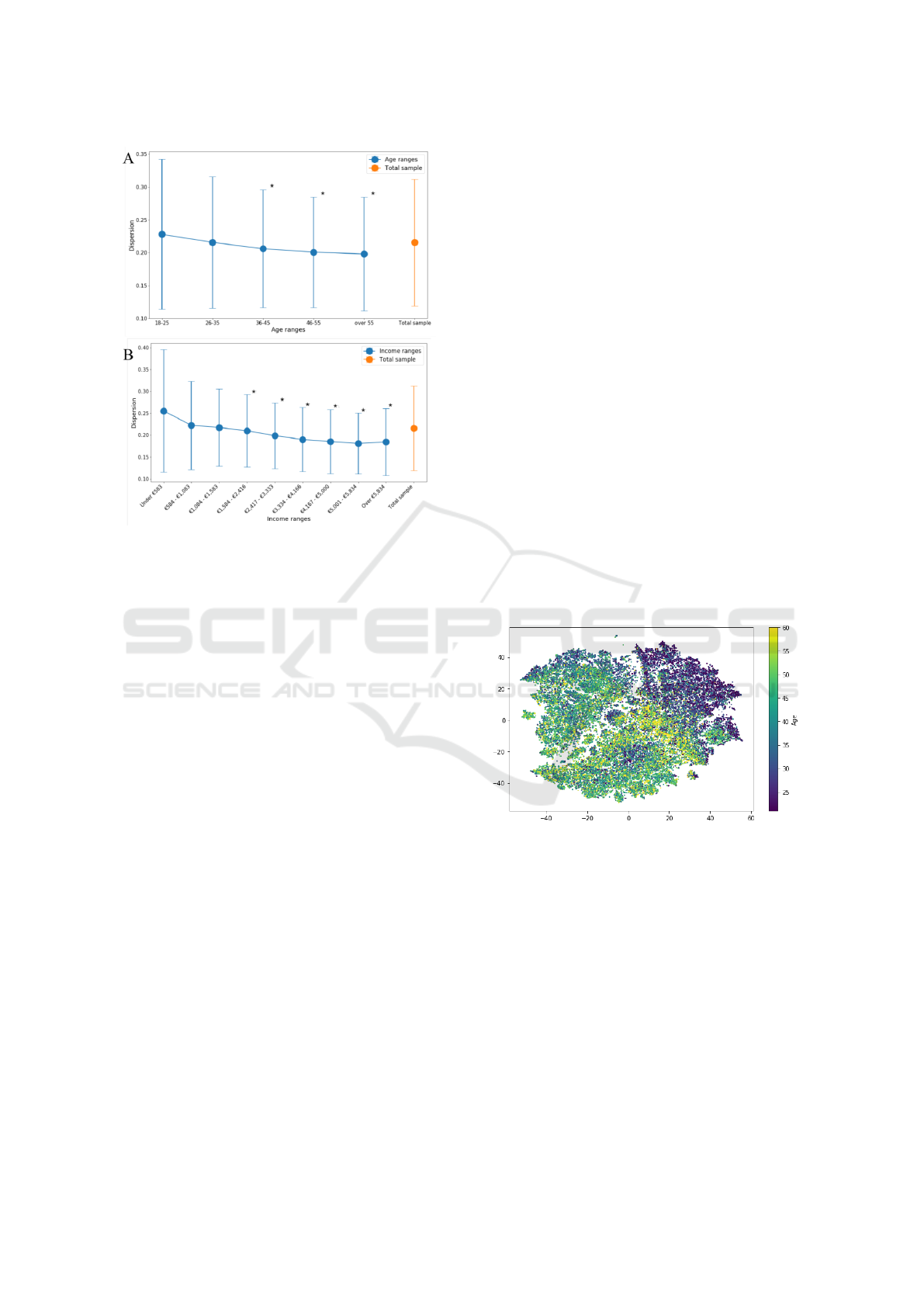
Figure 5: Distribution of dispersion within demographic
groups overlaps the distribution of dispersion of the total
sample. Dispersion measured as euclidean distance be-
tween all the users’ spending profile to the average spend-
ing profile. Orange: Dispersion of the total sample and
blue: dispersion within slices. A) Dispersion within age
ranges. B) Dispersion within income ranges. Error bars rep-
resent standard deviation. Significance of statistical test—
one sided Student-t—denoted as follows: * p-value <0.05.
mum variance. This traditional approach may be not
ideal when data structure cannot be fully explained
by linear projections–spirals are paradigmatic cases
of this limitation. As an alternative manifold learning
algorithms are a non-linear approach to perform di-
mensionality reduction. Considering a n-dimensional
space, manifold learning finds sets of data points
which are close to each other at the original high-
dimensional space. Once these sets are identified,
manifold learning reduces the dimensionality by em-
bedding the points into a lower-dimensional space,
while keeping the original structure and distances of
the points within those groups.
In this paper we used a particular manifold learn-
ing technique called t-SNE (Maaten and Hinton,
2008). Compared to other manifold learning algo-
rithms, t-SNE do not overlap points in the embed-
ded space, generating representations that easier to vi-
sualize. This technique maps any large-dimensional
vector into a low dimensional space using embed-
dings aiming to preserve relative distances between
points, as mentioned before. Thus, manifold learn-
ing allowed us to represent our 27-dimensional con-
sumption vector for each user as x,y coordinates of a
2-dimensional space.
In order to further confirm that demographic slices
are heterogeneous, we plotted the embedded x,y co-
ordinates as a 2D scatter plot. Since each point in
our plot represents each individual, we can color them
based on their age range (Fig. 6) or income range
(Fig. 7).
Although we can infer a larger concentration of
older individuals at the bottom left corner of the plot
and younger individuals at the top right corner, age
ranges are intertwined in this behavioral space (Fig.
6). The same is true when representing income ranges
age (Fig. 7). This representation visually confirms
our previous calculations on the heterogeneity of de-
mographic slices.
Extrapolating conclusions to the actual population
when using unsupervised embeddings is not trivial
and out of the scope of this paper. To be able to do
that extrapolation the sample data should mimic the
Spanish population. To do so we could either ran-
domly select a sub-sample that mimics the original
demographics, but that could mean discarding a large
part of our dataset. Or alternatively, we could artifi-
cially augment the under-sampled demographics, but
that would require a new set of assumptions about
those demographics.
Figure 6: t-SNE colored by age. Representation of the em-
bedding coordinates colored by user’s age range.
3.4 Using Manifold Learning to
Address the Problem
In previous sections, we confirmed that demographic
slices can be heterogeneous in terms of consump-
tion profiles. We also introduced the use of manifold
learning methods like t-SNE to visualize the whole
large-dimensional behavioral space. In this section,
we will show how we used the same t-SNE em-
bedding to generate more meaningful behavior-based
groups of individuals.
In order to visualize the individual consumption
across categories, we colored them by the budget
Manifold Learning to Identify Consumer Profiles in Real Consumption Data
27
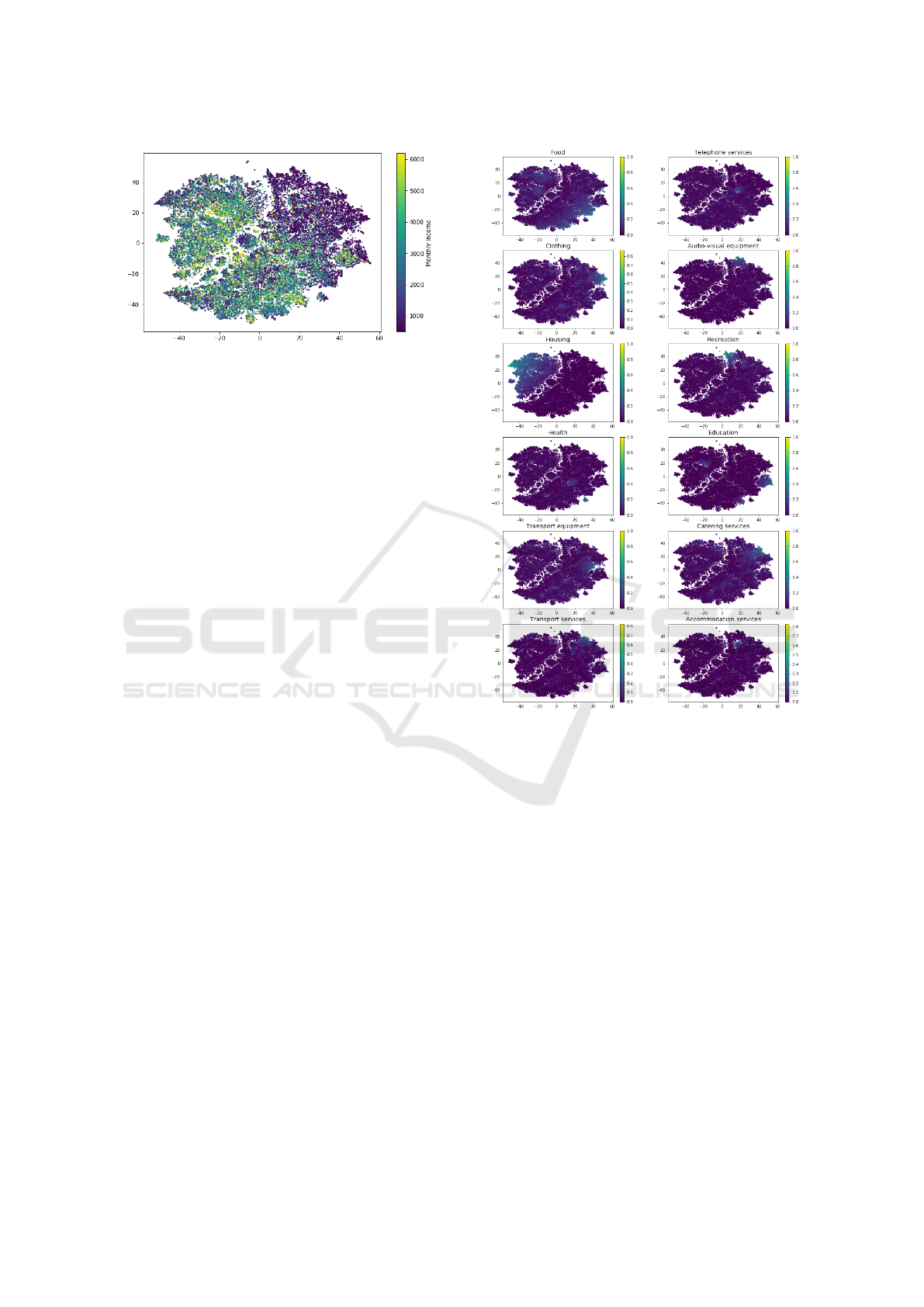
Figure 7: t-SNE colored by income. Representation of the
embedding coordinates colored by user’s income range.
share of each on a certain category (Fig 8) instead of
coloring the individual points by demographics slices.
As manifold learning tries to preserve relative dis-
tances between points, users who are close to each
other in this representation tend to have a similar con-
sumption profile.
Our implementation of t-SNE avoids the problem-
atic heterogeneity within demographic slices by con-
struction, since every user is represented. Moreover,
as data points aims to preserve their relative distances,
we can select behavior-based groups of users just by
vicinity. The members of each group share spend-
ing patterns and lifestyles, regardless of their demo-
graphic slices.
Following the strategy described above, we se-
lected two behavior-based groups from the embedded
space to further analyze them. We identified these
groups by selecting the nearest neighbours to some
relevant points—based on the euclidean distance be-
tween points in the embedded space. The first group
explored contains 300 users close to the top left cor-
ner of the space and therefore who spent a large bud-
get share on Housing. The second group analyzed
contains the 100 users closer to the top center part of
the plot and therefore showing a large relative spent
in Recreation. Second group have less users because
we confirmed graphical and analytically that due to
the density in the top center, 100 users are enough to
cover the area of interest. To confirm that the users
selected are in fact behaving as expected, we calcu-
lated the average consumption vector for each group
(Fig. 9).
One of our goals when computing groups using t-
SNE was to generate more homogeneous groups than
demographic slices. In section 3.3 we showed that the
dispersion of demographic slices overlapped with the
dispersion for the entire sample. So to test whether
we had in fact generated more homogeneous groups
we computed the dispersion within those groups and
we compared to the dispersion for the whole sample.
Figure 8: t-SNE colored by category budget share. Each
subplot represents the consumption ratio of every user on
the specific category.
The mean dispersion for both groups is statistically
smaller than mean the dispersion of the total sample;
Housing group dispersion: 0.14± 0.07 and Recre-
ation group dispersion: 0.16 ± 0.08 (Student-t test
for comparison of means with different standard de-
viations p −value < 10
−9
in both cases). This proves
that we have generated more homogeneous groups
than the total sample.
Once we have seen that our groups are homoge-
neous, we can further explore the characteristics of
the individuals in each of those new behavior-based
groups. In particular, we compared their demograph-
ics to the demographics of the total sample (see Ap-
pendix) to assay whether they show a different de-
mographic profile than the expected from the sample.
With this approach we found that individuals in the
Housing group are significantly more often middle
age than the total sample and less often young (bino-
mial tests, p −value < 0.01) (Fig. 10), but we did not
DATA 2019 - 8th International Conference on Data Science, Technology and Applications
28
observe relevant differences to the whole sample re-
garding income, region or gender. For the Recreation
group we also observed some statistical differences to
the sample. The members of this second group are
more often male (binomial test, p − value < 10
−6
),
at the youngest range (binomial test, p − value <
10
−19
) and at the lowest income range(binomial test,
p − value < 10
−20
) (Fig. 11).
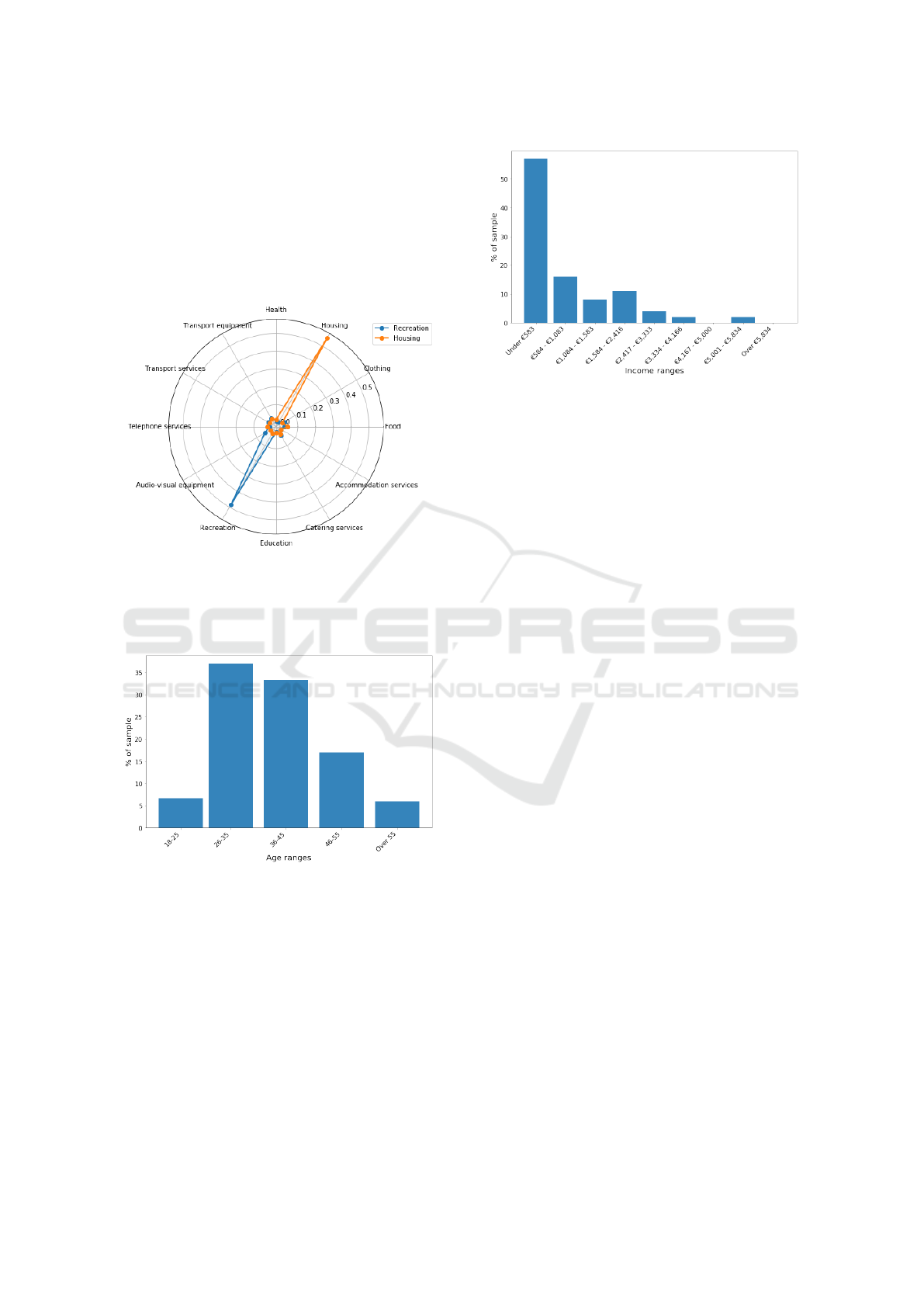
Figure 9: Slices of population selected from t-SNE. Blue
represent the average consumption profile of people who
mostly pay for Recreation and orange people who mostly
pay for Housing. Individuals were got from nearest neigh-
bours in the embedding matrix.
Figure 10: Age distribution from slice of individuals who
mostly pay for Housing. Bar height shows the percentage
of sample and horizontal axis the age range.
Although, the behavior-based groups derived from
the embedded visualizations could be composed
mostly of specific demographics, our unsupervised
method allow us to also include other individuals
that otherwise would be missed. Therefore, mani-
fold learning enhances on research by including data-
driven counter-intuitive insights into our analysis.
Figure 11: Income distribution from slice of individuals
who mostly pay for Recreation. Bar heights shows the per-
centage of the sample and horizontal axis the income range.
4 CONCLUSIONS
Precise analysis of people’s consumption can serve
as a basis to infer people’s preferences and needs.
To address this analysis, new technological develop-
ments open new opportunities for data collection al-
lowing us to generate new data sets as an alternative
to surveys. As these new data sets require new anal-
ysis methods, in this paper we propose the use of one
of these new methods—manifold learning—to embed
the multidimensional spaces of consumption profiles
into 2D spaces. This way, we generated meaningful
groups of individuals that transcends demographics.
The global adoption of electronic payments allow
the development of personal financial apps. These
apps generate micro-transaction databases that serves
us to build and analyze people’s consumption patterns
addressing some biases of the traditional approach:
household surveys. Furthermore, micro-transaction
data has more granularity that surveys, allowing us
to analyze individual by individual instead of house-
holds. These kind of data sets open a new field of
analysis opportunities to explore individual needs and
desires.
To analyze this new data set, we propose the use
of manifold learning to reduce the dimensionality of
consumption vectors in order to visualize the behav-
ior of thousands of individuals at the same time. This
visualization allowed us to find new consumption pat-
terns and lifestyles regardless of demographic groups.
The same technique can be use by marketers to under-
stand their clients and by policy makers to better assay
people’s behaviors and needs.
On top of better visualizations using manifold
learning we grouped individuals based on their con-
sumption profiles instead of standard demographic
Manifold Learning to Identify Consumer Profiles in Real Consumption Data
29

segments. Standard demographic segmentation show
intra-group heterogeneities regarding consumption
profiles that we reduced with our more homogeneous
behavior-based groups. The use of manifold learning
avoid biases by its non-supervised nature.
In this paper we showed that modern data sets
in conjunction with smarter big data analysis create
a powerful synergy to analyze peoples consumption,
needs and desires. A better understanding of individ-
uals behavior puts a step closer to more efficient poli-
cies towards a fairer world.
REFERENCES
Behrendt, C. E. (2005). Mild and moderate-to-severe copd
in nonsmokers: distinct demographic profiles. Chest,
128(3):1239–1244.
Cayton, L. (2005). Algorithms for manifold learning. Univ.
of California at San Diego Tech. Rep, 12(1-17):1.
Christian, L. (2012). Assessing the rep-
resentativeness of public opinion sur-
veys. Retrieved February 27th, 2019 from
http://www.people-press.org/2012/05/15/assessing-
the-representativeness-of-public-opinion-surveys/.
Council of European Union (2016). Regulation (eu)
2016/679 of the european parliament and of the coun-
cil of 27 april 2016 on the protection of natural per-
sons with regard to the processing of personal data and
on the free movement of such data, and repealing di-
rective 95/46/ec (general data protection regulation).
Official Journal of the European Union, L 119 (4 May
2016):1–88.
Deaton, A. (1997). The analysis of household surveys: a mi-
croeconometric approach to development policy. The
World Bank.
Deaton, A. (2001). Counting the world’s poor: problems
and possible solutions. The World Bank Research Ob-
server, 16(2):125–147.
Deaton, A., Muellbauer, J., et al. (1980). Economics and
consumer behavior. Cambridge university press, New
York, NY.
Deaton, A. and Zaidi, S. (2002). Guidelines for construct-
ing consumption aggregates for welfare analysis, vol-
ume 135. World Bank Publications.
Di Clemente, R., Luengo-Oroz, M., Travizano, M., Xu, S.,
Vaitla, B., and Gonz
´
alez, M. C. (2018). Sequences of
purchases in credit card data reveal lifestyles in urban
populations. Nature communications, 9.
Elgammal, A. and Lee, C.-S. (2004). Inferring 3d body pose
from silhouettes using activity manifold learning. In
Proceedings of the 2004 IEEE Computer Society Con-
ference on Computer Vision and Pattern Recognition,
2004. CVPR 2004., volume 2, pages II–II. IEEE.
Furnham, A. (1986). Response bias, social desirability and
dissimulation. Personality and individual differences,
7(3):385–400.
Groves, R. M. (2006). Nonresponse rates and nonresponse
bias in household surveys. Public opinion quarterly,
70(5):646–675.
INE (2017). Encuesta de Presupuestos Familiares. Madrid:
Instituto Nacional de Estadistica.
Jolliffe, I. (2011). Principal component analysis. Springer.
Maaten, L. v. d. and Hinton, G. (2008). Visualizing data
using t-sne. Journal of machine learning research,
9(Nov):2579–2605.
Morris, M., Evans, D., Tangney, C., Bienias, J., and Wil-
son, R. (2006). Associations of vegetable and fruit
consumption with age-related cognitive change. Neu-
rology, 67(8):1370–1376.
OECD/European Observatory on Health Systems and
Policies (2017). Spain: Country health profile
2017, state of health in the eu. Technical re-
port, OECD Publishing, Paris/European Observa-
tory on Health Systems and Policies, Brussels.
http://dx.doi.org/10.1787/9789264283565-en.
Pentland, A. S. (2013). The data-driven society. Scientific
American, 309(4):78–83.
Rogero-Garc
´
ıa, J. and Andr
´
es-Candelas, M. (2014). Fam-
ily and state spending on education in spain: Differ-
ences between public and publicly-funded private ed-
ucational institutions. Revista Espa
˜
nola de Investiga-
ciones Sociol
´
ogicas, 147:121–132.
United Nations, DESA (2018). Classification of Individ-
ual Consumption According to Purpose (COICOP)
2018. Statistical Papers, Series M No. 99,
ST/ESA/STAT/SER.M/99.
Wold, S., Esbensen, K., and Geladi, P. (1987). Principal
component analysis. Chemometrics and intelligent
laboratory systems, 2(1-3):37–52.
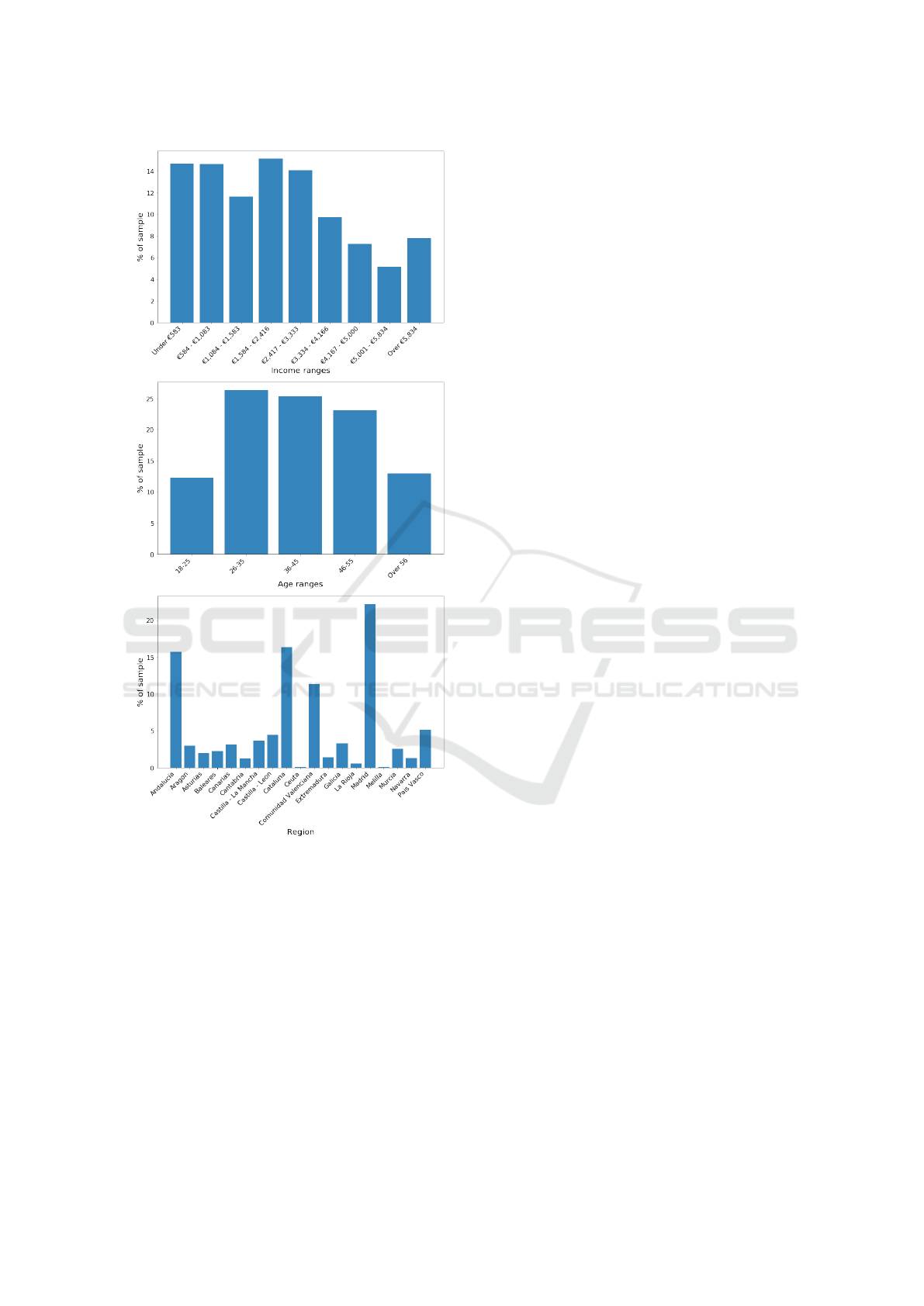
APPENDIX
Sample Demographics
Demographic distribution for the sample in the data
set for income ranges, age ranges and regions (Fig.
12). In addition, in our sample data we measured a
68% male ratio. These distributions are not meant to
be a representation of the Spanish population.
List of Categories
Complete list of 27 consumption categories. In bold
we highlighted the most relevant categories selected
for plotting through the paper:
• Health
• Housing
• Clothing
• Food
• Accommodation Services
DATA 2019 - 8th International Conference on Data Science, Technology and Applications
30
A
B
C
Figure 12: Demographic distributions of the sample. Bar
heights shows the percentage of the sample falling on a
given A) income-range, B) age-range or C) Region.
• Catering services—Restaurants and bars
• Education
• Recreation
• Audio-visual equipment
• Telephone Services
• Transport Services
• Transport Equipment
• Financial services
• Household appliances
• Other recreational items and equipment, gardens
and pets
• Personal care
• Insurance
• Electricity, gas and other fuels
• Water supply and miscellaneous services relating
to the dwelling
• Newspapers, books and stationery
• Other services n.e.c.
• Maintenance and repair of the dwelling
• Purchase of vehicles
• Tools and equipment for house and garden
• Goods and services for routine household mainte-
nance
• Social protection
• Furniture and furnishings, carpets and other floor
coverings
Manifold Learning to Identify Consumer Profiles in Real Consumption Data
31
