Optimal Trigger Sequence for Non-iterative Co-simulation

Franz Rudolf Holzinger

and Martin Benedikt

VIRTUAL VEHICLE Research Center, Inffeldgasse 21/A/II, Austria

Keywords:

Trigger Sequence, Execution Order, Calculation Order, Non-iterative Co-simulation, Travelling Salesman

Problem.

Abstract:

An execution sequence approach of interacting subsystem is presented for non-iterative co-simulation frame-

works. Local behaviour of coupling signals and subsystems are used to describe a general optimization prob-

lem of co-simulation. Therefore the linking matrix is weighted by analysis of the coupling signals within fuzzy

integrated expert knowledge. The weighted linking matrix is transferred to a directed co-simulation graph,

which can be interpreted as an appropriate travelling sales man problem. The solution of this co-simulation

graph provides an optimized trigger sequence of the subsystems.

1 INTRODUCTION

In the last decade co-simulation becomes a relevant

technique in diverse system development approaches,

especially in the automotive industry. The increas-

ing complexity of the systems forces engineers to di-

vide problems in several smaller sub-problems. These

subsystems are often modelled in speciﬁc simulation

environments and are solved by their own solvers.

Co-simulation is a technique to combine these sub-

models to an overall common system and allows

to run a holistic simulation (K

ubler and Schiehlen,

2000).

The increasing number of subsystems and cou-

pling signals in co-simulation presents a signiﬁcant

challenge for each co-simulation user and application

engineer. The individual subsystems and coupling

signals have different dynamic behaviour. These have

to be considered in the coupling by appropriate cou-

pling time steps of the several subsystems, proper

choice of extrapolation ﬁlters and suitable trigger se-

quence of the subsystems. In general, application en-

gineers have barely information about the subsystems

and so it is hardly possible to prepare a co-simulation

conﬁguration with respect to simulation duration and

simulation accuracy. Therefore it is necessary to sup-

port the co-simulation user by an automatically con-

ﬁguration of the co-simulation. This idea was al-

ready generally discussed by the authors (Benedikt

and Holzinger, 2016). An automated approach for ob-

https://orcid.org/0000-0003-3551-6579

https://orcid.org/0000-0003-2652-6812

taining the trigger sequence for co-simulation to im-

prove the simulation accuracy is discussed in the fol-

lowing.

The outline of this work is as follows. This pa-

per starts with an introduction into non-iterative co-

simulation. Reasonable information utilized for trig-

ger sequence determination is identiﬁed based on dis-

cussion on possible sources of coupling errors. An

approach to get a proper trigger sequence based on

the idea to solve travelling sales man problem is pre-

sented. This approach is illustrated and discussed by

an example.

2 NON-ITERATIVE

CO-SIMULATION

There are two well-established types of co-simulation

techniques: iterative and non-iterative. Compared to

iterative co-simulation the non-iterative one does not

allow to repeat a coupling step. In general this allows

a higher simulation performance in terms of simula-

tion duration. On the other hand the discretization

caused by the coupling mechanism is much higher.

Nevertheless the non-iterative co-simulation is com-

monly used in industry. Therefore one of the reasons

is that many simulation tools and subsystems do not

support external control reset of internal states and

thus repeating a time step is not possible.

In general, the induced coupling errors are higher

in the case of non-iterative co-simulation compared

to iterative co-simulation. Bidirectional dependencies

Holzinger, F. and Benedikt, M.

Optimal Trigger Sequence for Non-iterative Co-simulation.

DOI: 10.5220/0007833800800087

In Proceedings of the 9th International Conference on Simulation and Modeling Methodologies, Technologies and Applications (SIMULTECH 2019), pages 80-87

ISBN: 978-989-758-381-0

between subsystems cause causality problems and so

extrapolation ﬁltering is needed. Low order poly-

nomial extrapolation ﬁlters are generally used to es-

timate the input for the next simulation step. The

commonly used ﬁlter technique is the zero-order-hold

(ZOH) extrapolation. Here the last determined value

of the coupling signal is set as input signal during

the next calculation step. In addition to the error be-

tween the estimated signal and the actual determined

signal, the resulting staircase-shaped input signal can

also stimulate the subsystem and cause wrong results.

From the co-simulation conﬁguration point of

view, there are mainly three different kinds of options,

to inﬂuence and improve the simulation quality:

• Coupling step size to deﬁne how often signals are

exchanged between the subsystems

• Extrapolation ﬁlter to solve the causality problem

of bidirectional dependent subsystems

• Trigger sequence to deﬁne the calculation order of

the subsystems

The topics of extrapolation ﬁlter and coupling time-

steps were already well discussed in the past (Busch

and Schweizer, 2011) (Benedikt et al., 2010). There

are still methods which compensate the extrapolation

error (Benedikt and Hofer, 2013), (Benedikt et al.,

2013). However a proper trigger sequence prevents

or at least reduces coupling errors at (some) inputs.

3 TRIGGER SEQUENCE

Co-simulation typically applies parallel scheduling

scheme in which all subsystems are calculated in par-

allel. This approach has a high simulation perfor-

mance (in terms of simulation duration) because the

subsystems can be calculated in the same time. Nev-

ertheless every input signal has to be extrapolated and

so in each coupling signal an error is induced. To re-

duce the coupling error subsystems can be executed

in sequential order, i.e. each subsystem is calculated

after the other.

The challenge is to deﬁne a trigger sequence or

calculation order, which minimizes the coupling ef-

fects. The number of possible sequences factori-

ally increases with the number of subsystems. A

simple co-simulation example with m = 4 subsys-

tems (see Fig. 1) leads already to m! = 24 differ-

ent possible conﬁgurations with respect to the exe-

cution order. The induced coupling error and thus

the results change depended on the deﬁned trigger se-

quence. With increasing number of subsystems it is

(even for experienced co-simulation application engi-

Figure 1: Co-simulation Topology.

neers) hardly possible to deﬁne a well-deﬁned trigger

sequence.

The connection between the inputs u

and outputs

of subsystems in the co-simulation is mostly the

single information which is available for the conﬁg-

uration problem. This relation can be described with

the linking matrix:

u = L · y. (1)

The linking matrix L is an orthogonal matrix

of the

dimension n, where n is the number of connections

between the subsystems. The connections of the co-

simulation topology from Figure 1 can be rewritten as

follows:



















0 0 0 0 0 1

1 0 0 0 0 0

0 0 1 0 0 0

0 0 0 0 1 0

0 1 0 0 0 0

0 0 0 1 0 0



















, (2)

where u = [u

, u

, . . . , u

]

is the input vector and y =

, y

, . . . , y

]

represents the output vector. A fully

description of the co-simulation is given by this rela-

tion. Nevertheless this relation does not give any in-

formation about the dependencies between the several

subsystems. Therefore an other relation is needed,

which describes a formal relation between each sub-

system. Instead of the linking matrix L which de-

scribes the connection between inputs and outputs,

the matrix D describes the dependency of the sub-

systems themselves. This relation can be written as

follows:

D =



· L · S



. (3)

The matrix D is a m × m matrix and represents the

adjacency matrix, i.e. the dependency from one sub-

system to another. The matrices S and T are n × m

dimensional and describe the correlation between the

subsystems and the connections, where S describes

the allocation of the source y

to the subsystems and T

In order to ensure orthogonality for multiply connected

outputs, these outputs are duplicated, i.e. each output has

exactly one connection line.

Optimal Trigger Sequence for Non-iterative Co-simulation

the allocation of the target u

to the subsystems. The

columns represent the inputs of each subsystem and

the rows their outputs.

The linking matrix is a dependency description of

the connection, but it does not give any information of

the dependency of the subsystems. Regarding to the

trigger sequence the dependency of the subsystems is

more relevant.

The system dependency D of the co-simulation

topology from Figure 1 is given as follows:

D =







− 1 0 1

0 − 1 0

0 0 − 1

1 0 1 −







(4)

A more general description of the dependency matrix

D can be written as follows:

D =



· C · L · S



, (5)

with C as a diagonal matrix of weighted inputs

, c

, . . . , c

. With this additional weights c

it is pos-

sible to increase the relevance of several inputs y

and

thus to change the dependency between subsystems.

3.1 Extended TSP Problem

The co-simulation network can be interpreted as an

asymmetric, directed graph. The subsystems repre-

sent the nodes and the edges are the connections be-

tween the subsystems. The number of signals from

one subsystem to another weights the edge, and so

the number of extrapolated inputs. The co-simulation

graph is depicted in Figure 2. The nodes represent the

several subsystems from Figure 1 and the edges the

coupling signals between the subsystems.

Figure 2: Co-simulation Graph.

In this context the trigger sequence can be inter-

preted as a Hamiltonian cycle, where every node or

subsystem is exactly visited once. In the case that the

C is the identity matrix (i.e. all coefﬁcients in the di-

agonal c

i j

= 1), the value of the edges represents the

number of extrapolated inputs. If for example node

3 is visited (i.e. subsystem S

is calculated) the sum

of incoming edges represents the number of extrapo-

lated coupling signals for this subsystem. Regarding

to the adjacency matrix D that means the sum of the

node’s column, see (6).

D =







0 c

0 0 c

0 0 0 c

0 c







(6)

If the node 3 is already visited, the subsystem has cal-

culated and the results are available. There is no ex-

trapolation needed any more for these coupling sig-

nals, i.e. the row of the node has to set to zero, see

(7).

D =







0 c

0 0 c

0 0 0 0

0 c







(7)

The more nodes or subsystems are visited the more

coefﬁcients become zero and the less inputs have to

be extrapolated.

Based on the graph representation of the co-

simulation network, the optimal trigger sequence re-

sults from the shortest path between all nodes. A gen-

eral description of the optimization problem can be

written as follows:

min

∑

j\i



∑

k\I

k j



i j

(8)

The coefﬁcients c

i j

represent the value of the edges

and x

i j

is 0 or 1 according if a path or node is visited.

Starting from each row i, every column j is consid-

ered. The coefﬁcients c

k j

along the column j are ac-

cumulated up. Already visited nodes or columns I are

not considered.

Nowadays a typical co-simulation problem in-

cludes less than ten subsystems and so in general the

dimension of the adjacency matrix is lower than ten.

Therefore the brute-force solving strategy for the co-

simulation graph is sufﬁcient and can be solved with

low effort. With less than 5 nodes or subsystems

the brute-force solving method is faster than alterna-

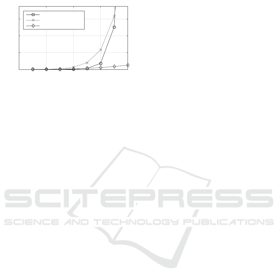
tive solving algorithms. The calculation effort of the

brute-force and other algorithm to solve the TSP prob-

lem is compared in Figure 3.

Nevertheless, with an increasing number of sub-

systems the calculation effort of the brute-force ap-

proach signiﬁcantly increases and so other solving

strategies with lesser computation effort should be

used.

SIMULTECH 2019 - 9th International Conference on Simulation and Modeling Methodologies, Technologies and Applications

0 2 4 6 8

Number of nodes

Calculation e,ort

Brute Force

Dynamic Programming

Nearst Neighbour

Figure 3: Calculation effort to solve a TSP problem.

However, it turns out that without any other in-

formation the subsystem within the lowest number

of inports should be calculated ﬁrst (Holzinger and

Benedikt, 2019).

It is obvious that, if no more information is avail-

able, the minimal number of extrapolated inputs is a

desirable goal for a trigger sequence. To ﬁnd this se-

quence the shortest way to connect all nodes has to

be found. The optimum trigger sequence can be de-

scribed as a modiﬁed travelling sales man problem

(TSP). In contrast to the original TSP, the (outgoing)

edges of already visited nodes have no impact to the

other nodes and thus these edges are set to zero.

3.2 Connection Properties

Depending on the relevance or impact of a connection

the weight of the signal c

i j

can inﬂuence the result

of the graph and consequently the trigger sequence.

This weighting can be inﬂuenced by different cou-

pling signal and subsystem properties (Benedikt and

Holzinger, 2016). In the following chapters some rel-

evant properties are discussed.

3.2.1 Subsequence

The subsequence is a subsystem property affected by

the subsystem solver, coupling time-step and the sub-

system interface. If the internal solving step size of a

subsystem, the so called micro step-size, is smaller

than the coupling step-size the subsystem provides

subsequence. Instead of a single value at the cou-

pling time-step, a sequence with the micro-steps is

given. These additional samples in the coupling sig-

nals generally allow more accurate simulation results

compared to single value coupling signals (coupling

time step equal micro time step).

3.2.2 Signal Types

The characteristic of the coupling signals is an impor-

tant information for the choice of a proper extrapo-

lation ﬁlter. The prediction of continuous signals is

easier than the estimation of a discontinuous or dis-

crete coupling signal. The most advanced extrapola-

tion and compensation techniques are based on con-

tinuous signal and so better to prevent the extrapola-

tion of discontinuous and discrete signals.

3.2.3 Direct Feed-through

The direct impact of an input to an output signal is one

of the most important properties of subsystem. Espe-

cially if the direct feed-through channels are formed

in a closed loop and affects an algebraic loop. An di-

rect feed-through indicates that an uncertainty at the

input signal (e.g. caused by an extrapolation ﬁlter)

means an uncertainty at the output signal. The ex-

trapolation of such inputs should be avoided.

3.2.4 Subsystem Dynamic

An other indicator for the extrapolation and trigger se-

quence of a subsystem is its dynamical behaviour. A

high system dynamic indicates that uncertainty at the

input of a system has a high impact to the output. And

on the other hand that low dynamic systems barely re-

act to any changes and discontinuities to the input. So

the extrapolation of inputs of slow input-output dy-

namics should be preferred instead of inputs of high

dynamic subsystems.

3.2.5 Coupling Signal Frequency

In addition to the system dynamic the frequency of the

coupling signal represents a further information for

the extrapolation ﬁlter setting and trigger sequence. It

is obvious that it is easier to extrapolate a signal with

low frequency components. However, coupling sig-

nals with high frequency components are not implic-

itly signals which should be prevented to extrapolate.

If the following system has a low pass characteristic,

high frequencies and uncertainty at the input signal

are not critical. The combined consideration of the

individual input-output dynamics and the signal fre-

quency determines if extrapolation shall be applied.

3.3 Contribution of Expert Knowledge

To combine the connection properties fuzzy logic is

used. The output of the fuzzy algorithm represents

the weight of the input signal c

i j

and for the inputs

the results of the signal quantities are used. Expert

Optimal Trigger Sequence for Non-iterative Co-simulation

Simulation Results

Subsequence

Signal Types

Feed-Through

Local Dynamics

Coupling Signal

Frequency

Subsystem Solver

···

Fuzzy Logic/ Expert Knowledge

i j

D = (T

· C · L · S)

Solve Optimization Problem

Set Co-Simulation Conﬁguration

{

, S

, ...

}

Figure 4: Schematic procedure to get the trigger sequence.

knowledge is used to describe rules and transfer the

properties of each coupling signal to a weight of the

co-simulation graph.

A schematic procedure to determine the trigger

sequence is shown in Figure 4. The procedure

starts with the results of a successfully simulated co-

simulation. The results are used for the signal analy-

sis, where the properties of the signals are computed,

like signal types, direct feed-through, etc. The in-

formation is merged into the fuzzy logic, where the

expert knowledge is integrated. The fuzzy algorithm

support a weight for every connection. The weighted

matrix delivers with the source and target transfer ma-

trix the adjacency matrix D, which is solved to get an

optimized trigger sequence.

In the case, that no results are available to calcu-

late the weight of the connections (e.g. after a new

conﬁguration), all coefﬁcients of the weighted matrix

C are set to a default value c

i j

= 1. The resulting de-

fault trigger sequence has minimized the number of

inputs to extrapolate.

4 EXAMPLE

The following section shows an example to demon-

strate the described approaches. Therefore three

strategies are used to determine trigger sequences.

The ﬁrst strategy considers the number of extrapo-

lated inputs. The second uses the property of direct

feed-through to determine the trigger sequence and

the third strategy or advanced strategy weights the

coupling signals by subsystem and signal behaviour.

The example consists of four subsystems S

, S

and S

which are connected to another as shown in

Figure 1. The subsystems S

, S

and S

are based

on an example in (Benedikt and Drenth, 2018). The

subsystems describe the behaviour of spring-damper-

mass systems. The additional model S

is a super-

posed controller, which controls the output y

of the

subsystem S

4.1 Subsystem Description

The four subsystems are solved with a ﬁxed-step size

solver (Euler) and a step size δT = 0.1 ms. The cou-

pling time steps is constant for all subsystems ∆T =

1ms. The extrapolation ﬁlters for all coupling signals

is set to ZOH.

The mathematical description of the several subsys-

tems is as follows:

4.1.1 Subsystem 1

The subsystem S

is a second order linear model with

one input u

and two outputs y = [y

, y

]

. The

parameters are set c = 1000 and J

= 0.1. There is

a direct feed-through d = 44.27 from the input u

x =

0 −

c −

x +





y =

c −

x +





(9)

4.1.2 Subsystem 2

The second subsystem describes a PI-controller with

the parameter k

= 100 and k

= 0.1 of the form:

˙x = k

· x +(r − u)

y = x +k

· (r − u)

(10)

The set value r = 10 and the initial states of all sub-

systems are zero.

4.1.3 Subsystem 3

The subsystem S

has two inputs u = [u

, u

]

and

an output y

. The model has an integrative be-

haviour, there is no direct feed-through from the in-

puts to the output. The parameter J

= 0.9.

˙x =

· x +



1 −1



y = x

(11)

SIMULTECH 2019 - 9th International Conference on Simulation and Modeling Methodologies, Technologies and Applications

S4S3S2S1

S4S3S1S2

S4S2S3S1

S4S2S1S3

S4S1S2S3

S4S1S3S2

S3S4S2S1

S3S4S1S2

S3S2S4S1

S3S2S1S4

S3S1S2S4

S3S1S4S2

S2S3S4S1

S2S3S1S4

S2S4S3S1

S2S4S1S3

S2S1S4S3

S2S1S3S4

S1S3S2S4

S1S3S4S2

S1S2S3S4

S1S2S4S3

S1S4S2S3

S1S4S3S2

Trigger Sequence Permutation

Objective Function

Default Strategy: Extrapolated Inputs

Default Strategy: Direct Feed-Through

Advanced Strategy

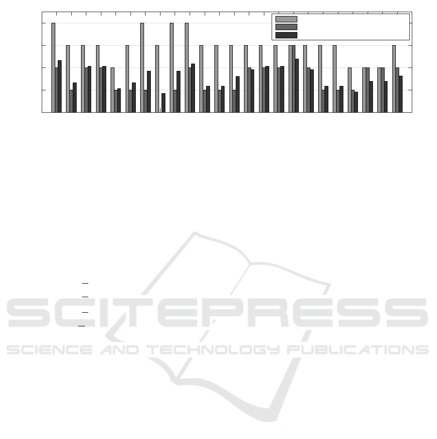
Figure 5: Evaluation of the objective function regarding different strategies: default strategy based on the extrapolated inputs,

default strategy based on the direct feed-through and advanced strategy.

4.1.4 Subsystem 4

The model S

has two inputs u = [u

, u

]

and two

outputs y = [y

, y

]

with a direct feed-through d =

44.27 from the input u

to y

and the parameter are

set c = 1000 and J

= 0.5.

x =

0 −

c −

x +



0 1

−1 d



y =

c −

x +



0 d

0 0



(12)

4.2 Default Strategies

The default strategies describe the possibility to de-

ﬁne a trigger sequence without knowledge or with

reduced knowledge of the subsystem behaviours.

Therefore no additional analysis of the coupling sig-

nals is needed to determine a trigger sequence for the

subsystems.

4.2.1 Extrapolated Inputs

In a ﬁrst step without any additional information the

weight of all coupling signals is set to one, c

= 1, and

so the adjacency matrix D of the graph is given by (4).

In this case the linking matrix L is the single required

information to determine a trigger sequence. The

resulting trigger sequence represents the minimum

number of extrapolated inputs. The best solutions of

the default matrix are

{

, S

}

{

, S

}

{

, S

}

and

{

, S

}

. All of these so-

lution delivers a minimum according to (8). Each

for each of the resulting trigger sequences two inputs

have to be extrapolated in each simulation step.

4.2.2 Direct Feed-through

If the direct feed-through of a system is known by

the application engineer, this information can be

used as prior knowledge to deﬁne a trigger sequence.

Some subsystems also provide this information, e.g.

the FMI standard supports the information of direct

feed-through (Blochwitz et al., 2012).

The subsystems of the considered example have

three inputs with a direct feed-through to an output.

A reduced adjacency matrix D with the direct feed-

through is given as follows:

D =







− 1 0 0

0 − 0 0

0 0 − 1

1 0 0 −







, (13)

where each input with a feed-through to an output is

set to one. Based on the adjacency matrix D from

(13) the best solution is

{

, S

}

. The resulting

trigger sequence represents the minimum number of

inputs with a direct feed-through to an output. In the

example exits one conﬁguration, where no input with

a direct feed-through has to be extrapolated.

4.3 Advanced Strategy

By the advanced strategy the default weights are mod-

iﬁed based on the identiﬁed connection properties.

The adjacency matrix D can be rewritten as follows:

D =







− 1 0 0.35

0 − 0.25 0

0 0 − 0.72

0.67 0 0.25 −







(14)

The integrative behaviour of subsystem S

reduces the

coefﬁcients c

= c

= 0.25. On the other hand, the

Optimal Trigger Sequence for Non-iterative Co-simulation

coefﬁcients c

and c

of the coupling inputs with

direct feed-through behaviour are still high.

The cost to solve the objective function for all pos-

sible trigger sequences with respect to the three dis-

cussed strategies are illustrated in Figure 5. The two

default strategies show the evaluation of the objec-

tive function based on the minimum number of ex-

trapolated inputs with respect to (4) and the minimum

number of extrapolated direct feed-through channels

with the adjacency matrix (13). The advanced strat-

egy show the results of (14). The best solution deliv-

ers the trigger sequence

{

, S

}

The default strategy based on the direct feed-

through and the advanced strategy provides the same

trigger sequence. This is due the fact, that the sub-

system properties are mainly characterized by the di-

rect feed-through. Nevertheless, in examples with

more coupling signals or if the property of direct feed-

through is not known, the presented (advanced) ap-

proach helps to get a proper trigger sequence.

The determined solution

{

, S

}

is not

from the optimal set, which was calculated with

the default strategy based on the minimum number

of extrapolated inputs

{

, S

}

{

, S

}

{

, S

}

and

{

, S

}

. The solutions

from the default strategy have a minimal number of

extrapolated inputs, but all of the solutions extrap-

olate an input signal of a subsystem with a direct

feed-through property. The direct feed-through can

be interpreted as an additional extrapolation of corre-

sponding output signal and will cause additional cou-

pling errors.

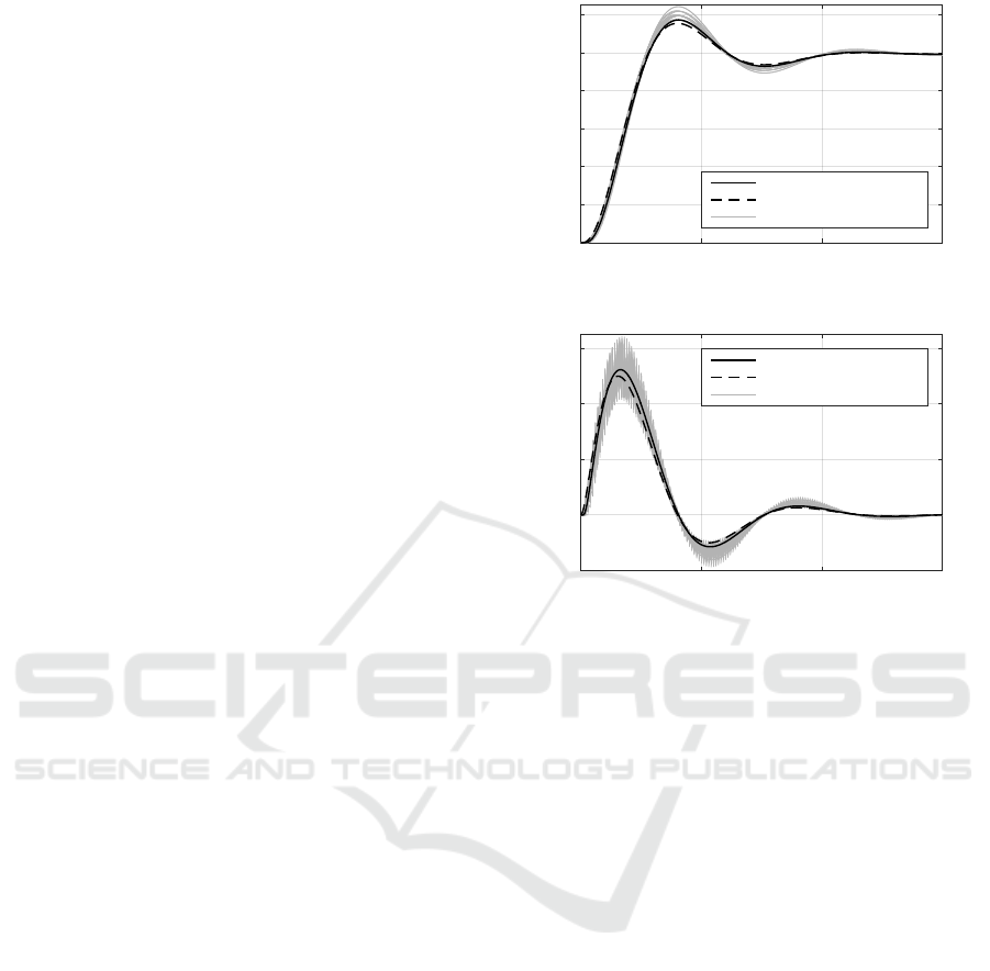
The results of the subsystem S

are shown in Fig-

ure 6. The dashed plot in both ﬁgures represents the

monolithic simulation result, where all subsystems

were simulated assembled and with one solver in a

single simulation environment. The grey lines show

the results of all possible permutations of the trigger

sequence. The black solide line is the result of the

trigger sequence

{

, S

}

from the presented

approach.

The result of the determined trigger sequence is

next to the monolithic simulation and has smaller

difference compared to the remaining permuted se-

quences. In the determined solution no input with di-

rect feed-through behaviour was extrapolated and so

the coupling error was reduced although that an ad-

ditional input has to be extrapolated compared to the

default solutions.

The other way around the solutions with high ef-

forts depicts a discrepancy to the monolithic solu-

tion. Nevertheless, even the best solution show dis-

crepancy between the monolithic solution caused by

the delay of the extrapolation ﬁlter. To compen-

0 0.05 0.1 0.15

Simulation Time in s

, y

Optimal Trigger Sequence

Monolithic Simulation

Permuted Trigger Sequence

0 0.05 0.1 0.15

Simulation Time in s

-20

, y

Optimal Trigger Sequence

Monolithic Simulation

Permuted Trigger Sequence

Figure 6: Simulation results of the permutation, monolithic

simulation and the optimal trigger sequence {S

, S

sate these remaining difference advanced extrapola-

tion techniques can be used (Benedikt and Hofer,

2013) (Benedikt et al., 2013).

The presented approach provides an optimized

trigger sequence for sequential co-simulation. Nev-

ertheless it is obvious that the simulation duration for

sequential co-simulation is higher compared to par-

allel co-simulation, where each subsystem can cal-

culate at the same time. On the other hand, gener-

ally, sequential co-simulation delivers better simula-

tion results, due the fact, that less inputs have to be

extrapolated. Hierarchical co-simulation is a method

to get a trade-off between simulation accuracy from

and simulation duration. A conﬁguration approach

for hierarchical co-simulation based on the number of

extrapolated inputs and calculation effort of the sev-

eral subsystems was already discussed by the authors

(Holzinger and Benedikt, 2019).

5 CONCLUSIONS

The article addresses an approach to determine

an optimized trigger sequence for non-iterative co-

simulation. Therefore expert knowledge e.g. in form

of fuzzy rules is used to assess the extrapolation qual-

SIMULTECH 2019 - 9th International Conference on Simulation and Modeling Methodologies, Technologies and Applications

ity of each input, based on the properties of the cou-

pling signals. The so resulting weighted connections

are used to describe a co-simulation graph. The so-

lution of the graph delivers an optimized trigger se-

quence.

If no additional information in terms of simulation

results is available to calculate the connection proper-

ties, the approach delivers a default solution related

to the minimum number of extrapolated coupling sig-

nals. After each simulation run the simulation results

can be used to calculate the connection properties and

ﬁnally weight the graph to get an optimal trigger se-

quence. This information can also be used to set the

time-step and the extrapolation ﬁlter or at least to as-

sess the co-simulation.

In a further work, the presented approach will

be extended for the conﬁguration of hierarchical co-

simulation, so that some subsystems can be calcu-

lated in parallel and others sequentially. This allows a

trade-off between simulation accuracy and simulation

duration.

REMARK PATENT

The presented work describes a part of a novel au-

tomatic conﬁguration approach for co-simulation of

distributed components. Protected by a pending Eu-

ropean patent (Benedikt et al., 2016) the outlined

schemes are supported by the co-simulation platform

Model.CONNECT

(AVL, 2018) from AVL.

ACKNOWLEDGMENT

This work was accomplished at the VIRTUAL VE-

HICLE Research Center in Graz, Austria. The au-

thors would like to acknowledge the ﬁnancial sup-

port of the COMET K2 - Competence Centers for

Excellent Technologies Programme of the Austrian

Federal Ministry for Transport, Innovation and Tech-

nology (bmvit), the Austrian Federal Ministry of Sci-

ence, Research and Economy (bmwfw), the Austrian

Research Promotion Agency (FFG), the Province of

Styria and the Styrian Business Promotion Agency

(SFG).

REFERENCES

AVL (2018). Model.CONNECT

, the neutral model inte-

gration and co-simulation platform connecting virtual

and real components. (https://www.avl.com/-/model-

connect). [Online; accessed 31.01.2019].

Benedikt, M., Bernasch, J., Holzinger, F., and Watzenig, D.

(2016). Method for conﬁguration a co-simulation for

a total system. EP3188053 (A1) — 2017-07-05.

Benedikt, M. and Drenth, E. (2018). Relaxing stiff sys-

tem integration by smoothing techniques for non-

iterative co-simulation. In IUTAM Symposium on Co-

Simulation and Solver-Coupling.

Benedikt, M. and Hofer, A. (2013). Guidelines for the ap-

plication of a coupling method for non-iterative co-

simulation. In Modelling and Simulation (EUROSIM),

2013 8th EUROSIM Congress on, pages 244–249.

Benedikt, M. and Holzinger, F. R. (2016). Automated con-

ﬁguration for non-iterative co-simulation. In 2016

17th International Conference on Thermal, Mechan-

ical and Multi-Physics Simulation and Experiments

in Microelectronics and Microsystems (EuroSimE),

pages 1–7.

Benedikt, M., Stippel, H., and Watzenig, D. (2010). An

adaptive coupling methodology for fast time-domain

distributed heterogeneous co-simulation. In SAE 2010

World Congress and Exhibition. SAE International.

Benedikt, M., Watzenig, D., Zehetner, J., and Hofer, A.

(2013). Macro-step-size selection and monitoring of

the coupling errof for weak coupled subsystems in the

frequency-domain. In Proceedings, pages 1–12. .

Blochwitz, T., Otter, M.,

Akesson, J., Arnold, M., Clauss,

C., Elmqvist, H., Friedrich, M., Junghanns, A.,

Mauss, J., Neumerkel, D., Olsson, H., and Viel,

A. (2012). Functional mockup interface 2.0: The

standard for tool independent exchange of simulation

models. In Proceedings of the 9th International Mod-

elica Conference, pages 173–184. The Modelica As-

sociation.

Busch, M. and Schweizer, B. (2011). An explicit approach

for controlling the macro-step size of co-simulation

methods. In Bernadini, D., editor, Proceedings of

the 7th European Nonlinear Dynamics Conference

(ENOC 2011): July 24 - 29, 2011, Rome, Italy, pages

1–6.

Holzinger, F. R. and Benedikt, M. (2019). Hierarchi-

cal Coupling Approach Utilizing Multi-Objective Op-

timization for Non-Iterative Co-Simulation, volume

1348, pages 735–740.

ubler, R. and Schiehlen, W. (2000). Modular simulation

in multibody system dynamics. Multibody System Dy-

namics, 4.

Optimal Trigger Sequence for Non-iterative Co-simulation