Drive Chain Friction Characterization of a 6DOF Parallel Kinematics
Robot
Hermes Giberti
1 a
, Francesco La Mura
1 b
, Ivan Raineri
2
and Marco Tarabini
2
1
Universita’ degli Studi di Pavia, Dipartimento di Ingegneria Industriale e dell’Informazione,
Via A. Ferrata 5, 27100 Pavia, Italy
2
Politecnico di Milano, Department of Mechanical Engineering, Campus Bovisa Sud, via La Masa 1, 20156 Milano, Italy
Keywords:
Ball-screw, Friction, PKM, Robot, Stribeck, Axis, Practical Approach, Stick Slip.
Abstract:
This paper describes a time-efficient method for friction characterization on a Robot drive chain, namely
a Ball-screw transmission. The Method promotes practical application by being independent from external
sensors and giving very precise and usable output model. A complete extimation procedure is described
togheter with the results obtained on the real Machine.
1 INTRODUCTION
This article describes the friction model identification
methods used on the drive chain characterization of a
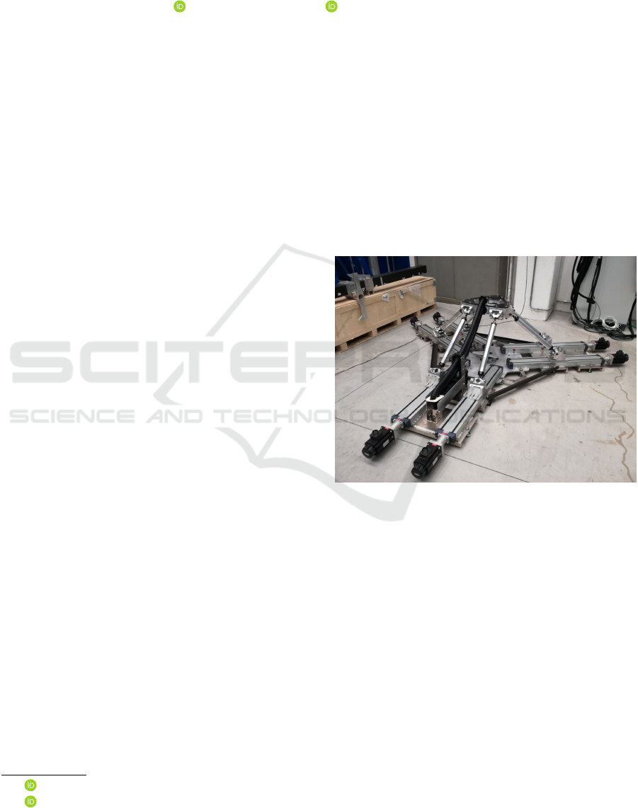
6DOF PKM. The case study of this work deal with the
ball-screw drive o a parallel kinematics robot named
Hexafloat, shown in fig.1.
An HIL (Hardware-In-the-Loop) architecture, re-
quiring high dynamics, performances and safety, is
deputed to simulate the ecosystem of an off-shore
wind turbine. Hexafloat machine has to carry the
scaled model of a floating wind turbine, and repli-
cate the behaviour of its floating platform inside the
wind gallery thanks to a complex real-time force con-
trol loop (Bayati et al., 2014; Bayati et al., 2017; Fer-
rari and Giberti, 2014; Fiore et al., 2016; Giberti and
Ferrari, 2015; Giberti et al., 2018). For many safety
and performance related reasons, a digital replication
(Digital-Twin (Raineri et al., 2018)) of this robotic de-
vice as been created with the goal to preliminary test
the architecture, develop control strategies (La Mura
et al., 2018b; La Mura et al., 2018a) and check for
control issues and performances lack (Silvestri et al.,
2011; Confalonieri et al., 2018). In order to obtain
Digital-Twin behaviour matches real device perfor-
mances, accurate friction description is crucial.
Ball-screw direct coupling with Servo-Motor is an
largely adopted solution in industrial field as well in
robotics. Due to the optimal trade-off between preci-
sion and cost, they are often preferred to linear mo-
tors and belt transmissions given the lower energy ef-
a
https://orcid.org/0000-0001-8840-8497
b
https://orcid.org/0000-0001-5143-7120
Figure 1: The Hexafloat: a 6DOF PKM.
ficiency of the former and the excessive deformability
of the latter (Negahbani et al., 2016).
As empirical evidence witnessed, friction com-
pensation is fundamental to improve the control per-
formance of ball-screw mechanisms.
Olaru et Al. (Olaru et al., 2004) exploited roll
contact theory with a modified Columbian model to
provide an estimate of friction. Successive analysis
carried out by Xu et Al. in (Xu et al., 2015) results
in a creep friction model based on contact rheology
which produces higher degree of accuracy for friction
identification.
In real world applications however, system fric-
tion characterization often overlaps with system con-
trol. To this end, different strategies can be imple-
mented and, to cope with increasing requirements of
position accuracy, new and complex friction models
have come to light. Frequency domain approaches
Giberti, H., Mura, F., Raineri, I. and Tarabini, M.
Drive Chain Friction Characterization of a 6DOF Parallel Kinematics Robot.
DOI: 10.5220/0007837806330640
In Proceedings of the 16th International Conference on Informatics in Control, Automation and Robotics (ICINCO 2019), pages 633-640
ISBN: 978-989-758-380-3
Copyright
c
 2019 by SCITEPRESS – Science and Technology Publications, Lda. All rights reserved
633

include the Differential Binary Squared Input as in
(Chen et al., 2002) and the limit cycle analysis pre-
sented in (Kim and Chung, 2006). According the
time domain approaches, Lee et al. (Lee et al., 2015)
proposed a PD feed drive position controller with
observer-based friction compensator, Ro et al. (Ro
et al., 2000) used a PD feed drive position controller
with disturbance observer while Maeda and Iwasaki
(Maeda and Iwasaki, 2013) developed an initial fric-
tion compensator. Keck et Al. (Keck et al., 2017)
put forward an interesting identification methodol-
ogy while applying feed-forward friction compensa-
tion based on Elasto-Plastic model. The aforemen-
tioned works address micro-positioning but, in many
applications, the minimization of Steady-State error,
although desirable, isn’t a priority. If this is the case,
the possibility to select a simpler, but yet physically
meaningful, friction model whose parameters can be
easily estimated is enticing. This holds especially
true when ball-screw characterization is an aspect of
a wider picture.
This paper aims at proposing a new, practical
method to characterize friction in ball-screw actua-
tors, developing and refining previous ideas find in
literature (Keck et al., 2017). The method will be in-
dependent from external sensors while having an op-
timized test total time and cost. Thanks to a suited ex-
perimental campaign, a peculiar friction induced phe-
nomenon has been observed and estimated. The influ-
ences of the so called Stick-Slip effect on the overall
friction behaviour led to the selection of three friction
models with increasing complexity; with the objec-
tive to describe comprehensively the overall frictional
trend. Parameters identification is performed for each
model while pro and cons are highlighted.
2 SYSTEM MODELING
The robot is made of 6 identical kinematic chains,
each of which composed by two passive universal
joints, a link with free a mechanism that allows free
axial rotation, a carriage holding one of the univer-
sal joint and a drive chain. Each drive chain is made
by three main components as depicted in Fig 2: a) A
brushless motor, that provides the torque; b) A tor-
sionally rigid coupling, that transmits torque from the
motor shaft to the ball-screw; c) Ball-Screw, it trans-
forms rotary motion into linear motion and carries the
load attached to the nut. It’s the main responsible for
friction losses.
Admitting the hypothesis of rigid bodies, it is pos-
sible to transform the system in an equivalent SDOF
translating system. The second order differential dy-
Figure 2: Main components of a ball-screw actuator.
namic equation ruling the system is:
M
equivalent
¨x = F
motor
− F
f riction
(v) − F
load
(1)
Being F
motor
=
C
motor
τ
with τ the transmission rate. In
the case of ball-screw τ = [
m
rad
] =
lead
2π
. Let’s now im-
pose a zero load condition F
load
= 0 for the sake of
identification by disconnecting the transmission from
the other robot components. Additionally, the equa-
tion at equilibrium ¨x = 0, offers a useful representa-
tion as in Eq 1:
0 = F
motor
− F
f riction
(v) ⇒ F
motor
= F
f riction
(v) (2)
It is thus possible to use a constant velocity motion
law to exploit Eq 2 and map the F
f riction
through
F
motor
. A displacement motion law, created append-
ing various ramps with different slopes, can test fric-
tion force for velocities corresponding to the slope of
each ramp.
3 PROPOSED METHOD
The proposed method articulates in four phases: 1)
creation of a suitable test motion law; 2) execution
of the aforementioned motion law and collection of
servo-motor torque signal; 3) data-set batch process-
ing; 4) Identification of parameters for the different
friction Models. The main idea behind this procedure
is to feed the controller with a reference displacement
made up of ramps and rests, collect the servo-motor
torque readings and obtain the mean value of motor
action for each tested velocity.
3.1 Friction Models
Among many different possibilities, pursuing a
proper balance between model complexity and com-
pleteness, three friction models are selected: Stribeck
model, modified Stribeck model and Neural Network
(NN) model.
Stribeck: In presence of lubrication, friction force
can be described with Stribeck Model as in Fig 3
It features a smooth and continuous transition from
the static region to the dynamic region. This model
is completely described by a set of 9 parameters:
[F
+
s
,F
+
c
,F
+
v
,v
+
s
,F
−
s
,F
−
c
,F
−
v
,v
−
s
,δ]. They are respec-
tively: F
s
is the Static friction force (this represents
ICINCO 2019 - 16th International Conference on Informatics in Control, Automation and Robotics
634

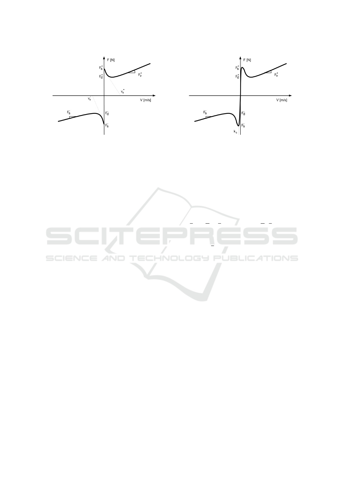
Figure 3: Stribeck friction.
the maximum force opposing the motion when system
is at rest), F
c
is the Columbian friction force (the mini-
mum force opposing the motion when system is mov-
ing), F
v
is the Viscous component of the friction force
(it is proportional to the velocity), v
s
is the Stribeck
velocity (this is the parameter ruling the exponential
envelope of Stribeck curve) and δ is the additional pa-
rameter which shapes the exponential envelope.
Each of the parameters, except δ, takes different val-
ues depending on the sign of velocity so that a to-
tal number of nine parameters is reached. Extending
the Armstrong-H
´
elouvry formulation for negative and
positive signs, the analytical expression of Stribeck
effect is:

F
f
= F
+
c
+ (F
+
s
− F
+
c
)e
−(v/v
+
s
)
δ
+ F
+
v
v f or v > 0
F
f
= F
−
c
+ (F
−
s
− F
−
c
)e
−(v/v
−
s
)
δ
+ F
−
v
v f or v < 0
Having considered the wide variability of the delta
value throughout literature and the lack of general
rules to assume its value a priori, it was chosen to
include it in the parameter estimation for the sake of
completeness.
Modified Stribeck: Although theorized to enhance
simulation capabilities (Andersson et al., 2007), this
model features an additional parameter which rules
the envelope of a tan(h) function. The analytic de-
scription is:











F
f
= F
+
c
+ (F
+
s
− F
+
c
)e
−(v/v
+
s
)
δ
tan(k
s
v) + F
+
v
v
f or v > 0
F
f
= F
−
c
+ (F
−
s
− F
−
c
)e
−(v/v
−
s
)
δ
tan(k
s
v) + F
−
v
v
f or v < 0
As can be seen in Fig 4, the curve corresponds to the
Stribeck model excepts in the x neighbourhood of the
origin, where it tends to zero. This interval widens as
k
s
approaches to zero.
Neural Network: Neural Networks identification of-
fers a model through implicit variables.This approach
is interesting to identification needs since it can pick
Figure 4: Modified Stribeck friction.
up unmodeled peculiarities of the motor-ballscrew
system. Among them: directional anisotropy of the
ball-screw transmission, coupled vibration-friction
phenomena and non-Newtonian behaviour of lubri-
cant. On the other hand, the estimated parameters
could have no direct physical interpretation. How-
ever, assuming friction force F
f riction
(v) is a function
of velocity only, the diagram can be simplified. A
compact notation expressing the relationship between
input and output takes this shape:
u = σ(wv + b); F
f riction
= σ(w
0T
u + b
0
)
(3)
where w and w
0
are the weights vectors and represents
connection importance between two neurons of dif-
ferent layers, u
j
is the activation state vector for hid-
den layer neurons, b and b
0
are the bias vectors con-
curring at activation state determination and σ is the
squashing or activation function.
3.2 Stick-Slip
The friction-induced Stick-Slip effect consists in a
jerky alternation of rest and motion phases. This phe-
nomenon manifests at low velocities with a cyclic
transition from dynamic to static condition and the
other way around. The presence of Stick-Slip may
modify macroscopically the friction nature approach-
ing the zero velocity region.
3.3 Test Motion Law
The first step to take in this phase is to select a set of
absolute values of velocities to test. In this effort, it is
advisable to generate the set by using a polynomial of
the type:
v
i
= a
0
+
J
∑
j=1
a
j
i
j
(4)
where v
i
is the i
th
element of the set and J is the order
of the polynomial. By opportunely choosing the de-
gree of the polynomial and the linear coefficients a
j
,
Drive Chain Friction Characterization of a 6DOF Parallel Kinematics Robot
635

it is possible to distribute the test velocities expedi-
ently. In general, it is preferable to test a bigger num-
ber of lower magnitude velocities, corresponding to
static-dynamic transition region, while consider less
high-magnitude velocities attaining the viscous effect
region characterized by a more constant slope. In a
second instance, an observation reference x = 0 is se-
lected, this position is preferably the midpoint of the
axis to avoid other phenomena affecting extreme axis
position and enhance travelling distances. Concur-
rently, an observation band is placed about the refer-
ence position. This band is suitable for discarding ac-
celeration and deceleration transient phases from ac-
quisition.
Right after, a motion law consisting of an alter-
nation of ramps and rest phases has to be generated.
The slope of the ramps is imposed by the velocities
set determined at the previous step. For each step,
both negative and positive sign should be considered
consequentially as suggested in (Keck et al., 2017).
Please notice that, as the magnitude of tested ve-
locity increases, the slider should travel further from
the observation band in order to guarantee that the
controller is able to enforce constant velocity during
the observation band cross-over. Position extremes to
be touched by the motion law in dependence from ve-
locity, as described by the following equation:

x
i+
= +q + m v f or v > 0
x
i−
= −q + m
i
v f or v < 0
where, at least, q
i
>
δx
i
2
. In order to guarantee
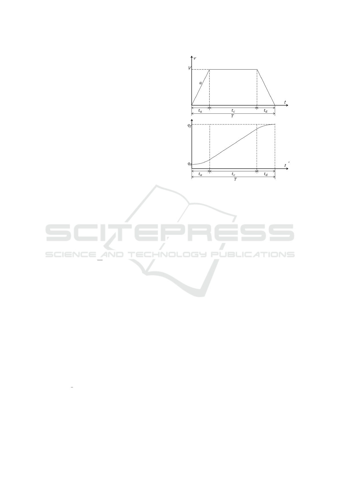
smoother transients, the ramp can be modified in a
symmetrical trapezoidal velocity profile. Aggressive
controls with relevant feed-forward contributions es-
pecially benefit from this practice. To implement such
a strategy, let’s consider the travel distance
q
f
= x
k+1
extreme
− x
k
extreme
the velocity to test V and the maximum acceleration
at disposal a. Trough the well known formulas of
trapezoidal motion law, shown in Fig 5, it is pos-
sible to build the motion law and estimate the total
time T needed to perform the smoothed ramp. After
each ramp, a rest phase of 1s, is observed to minimize
the influence of possible vibrations occurring in lower
stiffness systems at the end of the motion.
The sequence of ramps, with alternate slope
sign, and rests results in a motion law that hovers
around the observation reference, if initial condition
x
0
extreme
= ±
q
2
is assumed. It is now possible to con-
sider the sum of ramps and rests times composing the
motion law total time T
total
:
T
total
= T
total
(N, [a
0
,a
1
,...,a
J
],q,m,δx) (5)
Figure 5: Trapezoidal Motion Law.
As a function of the number of velocities N to test, the
coefficients of the polynomial a
j
, the couple (q,m)
and the observation band δx. While this function is
sensitive to each of these inputs, it is especially effec-
tive to adopt a multi-band approach with the aim to
minimize the total execution time T
total
. By consider-
ing narrower observation bands on the lower velocity
ramps, it is possible to significantly reduce T
total
while
maintaining wider bands for the faster ones in order to
represent them properly. In general, it is possible to
state that:
T
total
= (N,[a
0
,a
1
,...,a
J
],q,m,[δx
1
,δx
2
,...,δx
K
],g(i))
(6)
where [δx
1
,δx
2
,...,δx
K
] are the K bands and g(i) is a
function of the i
th
tested velocity ruling when a band
succeeds to another. By tuning those parameters it is
possible to save significant execution time.
Once the motion law is executed, it is useful to
verify that the controller is actually capable to cope
with the requirements so that actual velocity is al-
most identical to the reference one. If this require-
ment is satisfied, then the Servo-Motor data collected
during motion law execution can be trusted. Motor
action time history is sliced in buffers with differ-
ent ramp lengths. For each segment attaining to the
single ramp, only the section related to observation
band cross-over is considered. Mean is taken over
those intervals resulting in the motor average action
for each tested velocity across its proper observation
band. Those data constitute the foundation for identi-
fication. The velocity-force pairs can be plotted on a
graphic to provide visual feedback representation.
ICINCO 2019 - 16th International Conference on Informatics in Control, Automation and Robotics
636

3.4 Identification of Friction Model
Parameters
The final step of the proposed method consists in
identification of parameters. To this purpose, a LSQ
– Least Square – identification is put forward. The
mean residual square error e
RMS
can be considered as
a figure of merit of the identification. If the test ve-
locities selection has been carried out wisely, there
should be no need to introduce weights. To solve
the minimization problem, a genetic algorithm is de-
ployed since its low dependency from initial guess.
Depending on the tested velocity and on the pe-
culiarities of the system object of identification, it
is possible Stick-Slip effects acquisitions under cer-
tain velocity limit. Anyhow, those influences smooth
out as velocity increases. When the vibration pro-
duced by Stick-Slip is not negligible for some of the
tested velocities, actions should be taken accordingly
to the friction models chosen for identification. To
improve Stribeck model parameter estimation, it is
better to purge experimental data from Stick-Slip af-
fected samples, while Modified Stribeck model and
NN model can better pick up this peculiarity.
4 EXPERIMENTAL SETUP
As said in Section 2 and going into further techni-
cal details, the drive chain of Hexafloat in made of
a TH145 SP4 ball screw linear axis by Rollon, a
Toolflex 20M coupling and a RM88-K2K030C-BS2
servo motor by Omron.
The servo motor is provided with a 20bit high-
resolution incremental encoder that provides posi-
tion feedback to the controller with an accuracy of
131072
cnt
rev
= 3277
cnt
mm
. In the mean time, the con-
troller keeps a data log of the computed action during
motion execution.
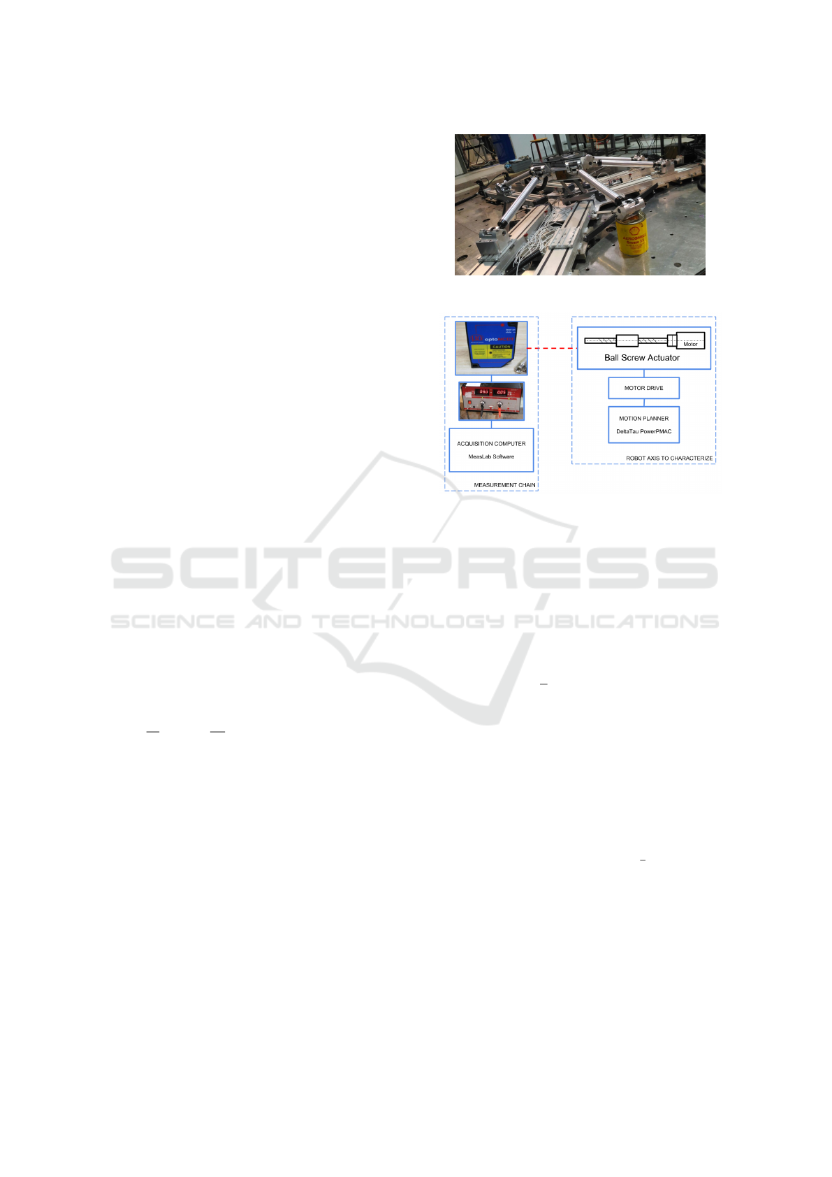
To the purpose of this experiment, robot leg is dis-
mounted from the slider to eliminate F
load
from eq.1.
This process is also unavoidable, since the parallel na-
ture of the robot, to safely move one slider at a time
with large displacements. Fig. 6 shows the leg disas-
sembled from the slider.
For the Stick-Slip phenomenon, a dedicated ex-
periment has been setup, using an external laser sen-
sor to measure local vibration of the slider when sub-
ject to low motor driving torques. During this exper-
iment, the sensor is positioned so that the slider can
move in a range of 4 mm without getting out of focus.
The measurement scheme is reported in fig 7.
Figure 6: Experimental Set-Up.
Figure 7: Experimental setup for Stick-Slip inquiry.
5 EXPERIMENTAL RESULTS
In this section the proposed method is applied. A
3
th
degree polynomial is used to generate the test
set with the coefficients hereafter summarized: a
0
=
100 × 10
−7
, a
1
= 100 × 10
−7
, a
2
= 40 × 10
−7
, a
3
=
3 × 10
−7
.
A total of N = 51 velocities exploring the interval
(0.02 − 50) × 10
−3
m
s
. Following the prescriptions re-
ported in 3.3, a first attempt motion law is designed
with an observation band δx = 10 mm. The gener-
ated motion law is excessively time consuming in the
first ramps. In order to minimize the total motion
law execution time T
total
, a three band approach is
adopted. The observation band value for each ramp
is described by: δx
1
= 2 mm for first three velocities,
δx
2
= 5 mm for the fourth, fifth and sixth velocity and
δx
3
= 10 mm for all the others.
The optimized motion law saves a considerable
time and results in a T
multi band
total
<
1
3
T
one band
total
. Fig
8 provides the graphical representation of multi-band
approach motion law.
Motion law is implemented inside robot motion
controller, for the axis object of the characterization.
During motion execution, the data log of control ac-
tion is registered as well as the actual position i.e. in-
ternal encoder measurements. The results on the latter
show that the controller can actually follow the ref-
erence as expected. The former is stored and keep
Drive Chain Friction Characterization of a 6DOF Parallel Kinematics Robot
637

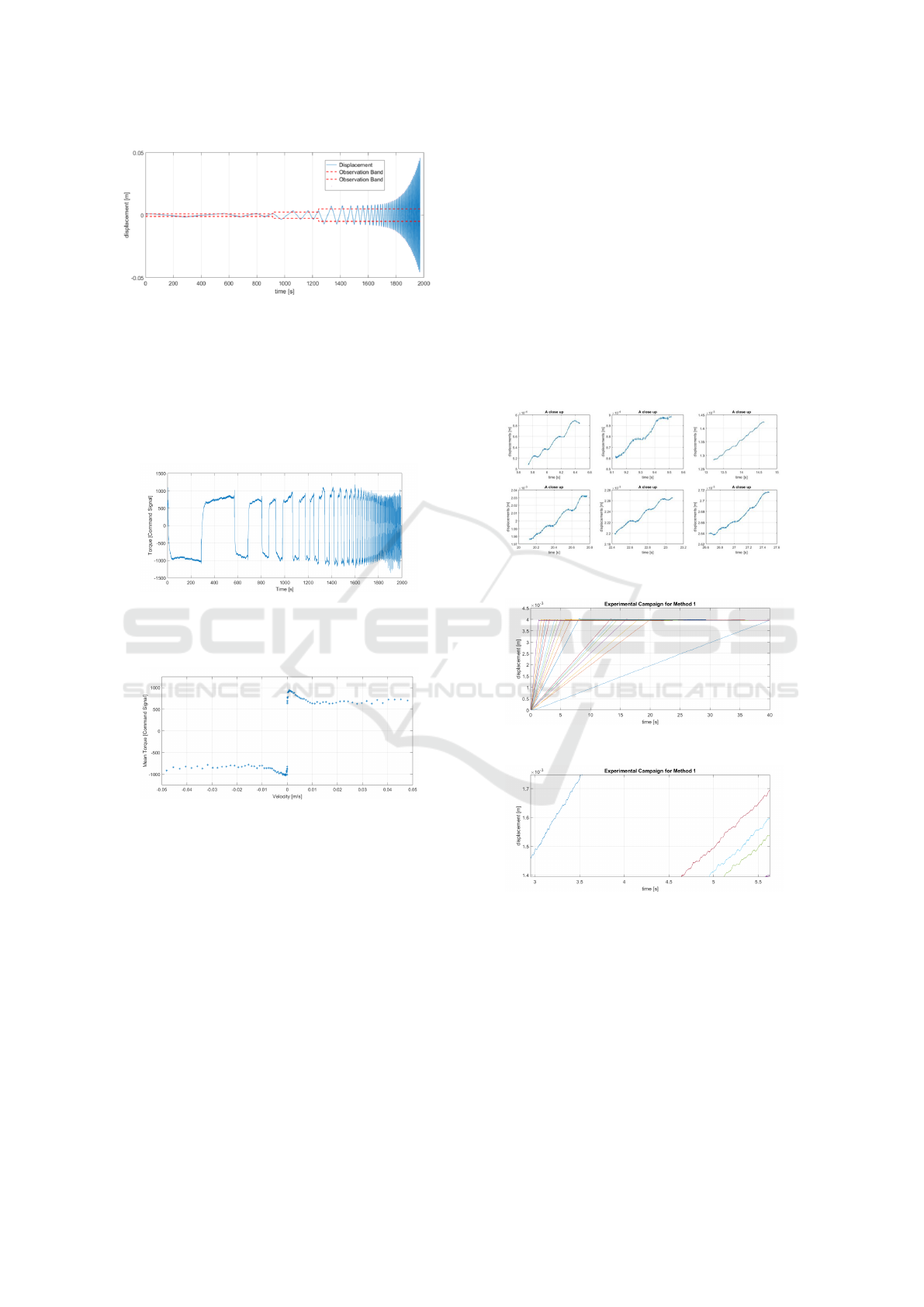
Figure 8: 1 Band vs 3 Bands approach, time comparison.
for further processing. Fig 9 displays the Reference
Motor Action time history. As can be noticed, when
the velocity changes from positive (upward ramp)
via zero (rest phase) to negative (downward ramp)
and vice-versa, the control effort undergo to signifi-
cant variations. Conversely, during ramp motion, the
change is considerably reduced.
Figure 9: Reference Motor Action.
After applying the averaging process described in
the 3.3, the velocity-force pairs are plotted in Fig 10.
Figure 10: Experimental Results. Velocity-
MeanMotorTorque pairs.
In a glance, it is possible to observe a general anal-
ogy with Stribeck curve. On the other hand, the points
related to low velocity ramps appear not to fit into the
normal Stribeck framework presented in 3.1. In par-
ticular, friction caused torque seams to lessen with re-
spect to ”static” equivalent value for a very narrow
velocity band around zero value. The next section ex-
plores this behaviour with insights on the stick-slip
phenomenon.
5.1 Stick-Slip Influence
As previously stated, Stick-Slip is a friction-induced
phenomenon occurring at low velocities. It consists
in a continuous transition from motion (slip phase)
to rest (stick phase) and vice-versa (Berman et al.,
1996). In order to better understand the influence of
this phenomenon on the axis dynamics, stick-slip in-
quiries are executed. For the sake of brevity and con-
sidering the supportive-only nature of this experiment
with respect to the method, we won’t dig into details.
Several tests are done and the motor is driven at differ-
ent constant velocities. A triangulation laser measures
the local displacement perturbations of the slider, re-
sulting from stick-slip induced vibrations. Fig. 11
shows an example of the phenomenon measured, fig.
12 reports the experimental campaign and fig. 13 a
detail of the previous, particularly important for the
discussion.
Figure 11: Measured Sick-Slip phenomenon.
Figure 12: Stick-Slip Experiments.
Figure 13: A Particular.
Analysing fig. 13, it is possible to notice a group
of three tests on the right and compare it to the one on
the left. As observed in the driving velocities range
of (0.5 − 0.3) × 10
−3
m/s, the influence of vibratory
phenomenon gradually smooths out. In this region is
no longer possible to clearly identify rest-slip phases
like in fig. 11. Although identification of a pre-
cise Stick-Slip critical transient velocity has not been
possible, it seems reasonable enough to consider this
speed within this band. For the sake of clarity from
now on this interval will be called Experimental Vi-
ICINCO 2019 - 16th International Conference on Informatics in Control, Automation and Robotics
638

bration Smoothing Interval. Switching back to the
preliminary result obtained in the previous section,
the following relation exists: all the points not fitting
the Stribeck model are related to ramps whose veloc-
ity is below the Vibration Smoothing Interval, while
for other acquisitions, no clear evidences of Stick-Slip
occurrence have been found.
Thus one can assume that microscopic vibration
induced by Stick-Slip reduces the macroscopic fric-
tion force. This hypothesis can be supported by
two different standpoint: a) A comparison can be
drawn with the control technique called high fre-
quency dithering; b) the microscopic entanglements
between surfaces do not bound effectively when dis-
turbed by a local vibration of the interfaces. To con-
firm this hypothesis further research are required.
Eliminating the data affected by Stick-Slip phe-
nomenon, one can refine the test results in the one de-
picted in Fig 14. Parameter estimation is performed
on those data.
Figure 14: Refined Test Result.
6 MODEL PARAMETERS
IDENTIFICATION
Parameter identification is carried out according to the
methodology exposed in section 3. The genetic algo-
rithm runs with an initial population of 10.000 indi-
viduals, maximum generation equal to 100 and a mu-
tation rate of 0.8. Additionally, the initial population
algorithm is endowed with a custom initial population
based on Divide-and-Conquer paradigm to enhance
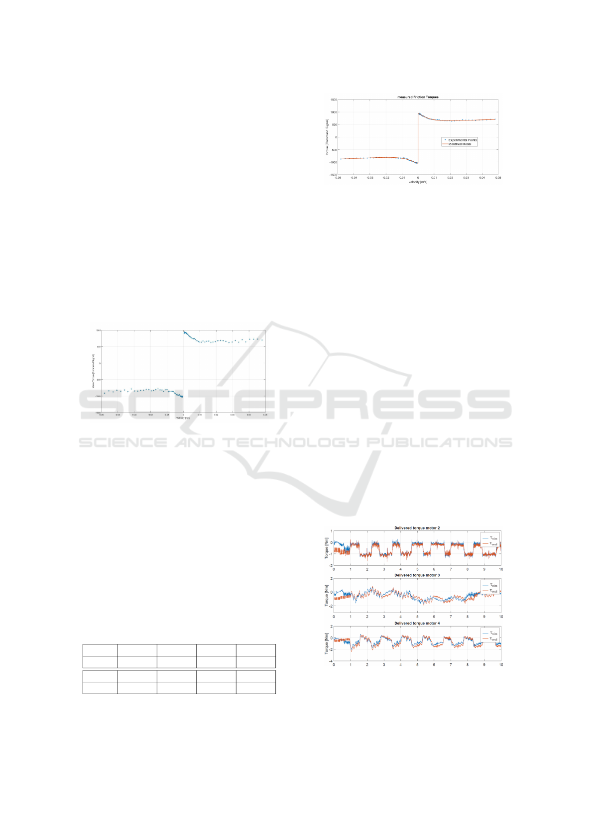
convergence efficiency. Results are satisfactory as can
be seen in Fig 15. Tab 1 reports the numerical values
for completeness sake.
Table 1: Identified Stribeck friction Parameters.
F
+
s
F
+
c
v
+
s
δ F
−
s
944.2 6111.8 0.0065 1.26 1049.2
F
−
c
v
−
s
F
+
v
F
−
v
e
RMS
750.9 0.0074 1904.2 2565.0 11.4
Figure 15: Identified Model.
7 CONCLUSIONS
In this article a simple and efficient friction estima-
tion methodology is proposed for the drive chain of a
PKM.
The proposed procedure successfully use servo
motor torque estimation and velocity measurements
to create velocity-force mapping, without the usage
of additional sensors and acquisition system over the
machine itself and it servo driver. The Stick-Slip phe-
nomenon has been also analyzed, together with its in-
fluence on acquired data and methods for extracting a
good model despite its effects. The model parameters
have been computed fitting experimental data with a
custom genetic algorithm and solving an LSQ prob-
lem. The results show a satisfactory match between
model and real data. This model is implemented in-
side the Digital Twin of the Hexafloat robot. Given
the exact same tool centre point position time history
as reference and the exact same control architecture
and gains, the command torque of the motors acquired
in both real and simulated case are shown in fig.16.
Results match satisfactory, even considering flexible
dynamics and other source of approximation inside
the digital replication of the machine that may lead to
very different actuators efforts.
Figure 16: Digital Twin command torque comparison with
real control effort.
Drive Chain Friction Characterization of a 6DOF Parallel Kinematics Robot
639

REFERENCES
Andersson, S., S
¨
oderberg, A., and Bj
¨
orklund, S. (2007).
Friction models for sliding dry, boundary and
mixed lubricated contacts. Tribology international,
40(4):580–587.
Bayati, I., Belloli, M., Bernini, L., Giberti, H., and Zasso,
A. (2017). Scale model technology for floating off-
shore wind turbines. IET Renewable Power Genera-
tion, 11(9):1120–1126.
Bayati, I., Belloli, M., Ferrari, D., Fossati, F., and Giberti,
H. (2014). Design of a 6-dof robotic platform for wind
tunnel tests of floating wind turbines. Energy Proce-
dia, 53:313–323.
Berman, A., Ducker, W., and Israelachvili, J. (1996). Ori-
gin and characterization of different stick-slip friction
mechanisms. Langmuir, 12(19).
Chen, Y.-Y., Huang, P.-Y., and Yen, J.-Y. (2002).
Frequency-domain identification algorithms for servo
systems with friction. IEEE transactions on control
systems technology, 10(5):654–665.
Confalonieri, M., Ferrario, A., and Silvestri, M. (2018).
Calibration of an on-board positioning correction sys-
tem for micro-edm machines. In EUSPEN Conference
Proceedings - 18th International Conference and Ex-
hibition, pages 153–154.
Ferrari, D. and Giberti, H. (2014). A genetic algorithm ap-
proach to the kinematic synthesis of a 6-dof parallel
manipulator. In 2014 IEEE Conference on Control
Applications (CCA), pages 222–227.
Fiore, E., Giberti, H., and Ferrari, D. (2016). Dynamics
modeling and accuracy evaluation of a 6-dof hexaslide
robot. In Nonlinear Dynamics, Volume 1, pages 473–
479. Springer.
Giberti, H. and Ferrari, D. (2015). A novel hardware-in-
the-loop device for floating offshore wind turbines
and sailing boats. Mechanism and Machine Theory,
85(Supplement C):82 – 105.
Giberti, H., La Mura, F., Resmini, G., and Parmeggiani, M.
(2018). Fully mechatronical design of an hil system
for floating devices. Robotics, 7(3):39.
Keck, A., Zimmermann, J., and Sawodny, O. (2017). Fric-
tion parameter identification and compensation us-
ing the elastoplastic friction model. Mechatronics,
47:168–182.
Kim, M.-S. and Chung, S.-C. (2006). Friction identifica-
tion of ball-screw driven servomechanisms through
the limit cycle analysis. Mechatronics, 16(2):131–
140.
La Mura, F., Roman
´
o, P., Fiore, E., and Giberti, H. (2018a).
Workspace limiting strategy for 6 dof force controlled
pkms manipulating high inertia objects. Robotics,
7(1):10.
La Mura, F., Todeschini, G., and Giberti, H. (2018b).
High performance motion-planner architecture for
hardware-in-the-loop system based on position-based-
admittance-control. Robotics, 7(1):8.
Lee, W., Lee, C.-Y., Jeong, Y. H., and Min, B.-K. (2015).
Distributed component friction model for precision
control of a feed drive system. IEEE/ASME Trans-
actions on Mechatronics, 20(4):1966–1974.
Maeda, Y. and Iwasaki, M. (2013). Initial friction compen-
sation using rheology-based rolling friction model in
fast and precise positioning. IEEE Transactions on
Industrial Electronics, 60(9):3865–3876.
Negahbani, N., Giberti, H., and Fiore, E. (2016). Error
analysis and adaptive-robust control of a 6-dof paral-
lel robot with ball-screw drive actuators. Journal of
Robotics, 2016.
Olaru, D., Puiu, G. C., Balan, L. C., and Puiu, V. (2004).
A new model to estimate friction torque in a ball
screw system. In Product engineering, pages 333–
346. Springer.
Raineri, I., La Mura, F., and Giberti, H. (2018). Digital twin
development of hexafloat, a 6dof pkm for hil tests.
In The International Conference of IFToMM ITALY,
pages 258–266. Springer.
Ro, P. I., Shim, W., and Jeong, S. (2000). Robust fric-
tion compensation for submicrometer positioning and
tracking for a ball-screw-driven slide system. Preci-
sion Engineering, 24(2):160–173.
Silvestri, M., Pedrazzoli, P., Bo
¨
er, C., and Rovere, D.
(2011). Compensating high precision positioning ma-
chine tools by a self learning capable controller. In
Proceedings of the 11th international conference of
the european society for precision engineering and
nanotechnology, pages 121–124.
Xu, N., Tang, W., Chen, Y., Bao, D., and Guo, Y. (2015).
Modeling analysis and experimental study for the fric-
tion of a ball screw. Mechanism and Machine Theory,
87:57–69.
ICINCO 2019 - 16th International Conference on Informatics in Control, Automation and Robotics
640