Small Radius Spheres in Output Space of Nonholonomic Systems
Arkadiusz Mielczarek and Ignacy Duleba
Dept. of Cybernetics and Robotics, Wroclaw University of Science and Technology, Janiszewski St. 11/17, Wroclaw, Poland
Keywords:
Nonholonomic System, Configuration Space, Output Space, Sphere, Motion Planning.
Abstract:
In this paper small radius spheres of driftless nonholonomic systems in an output space are analyzed. The
nonholonomic systems appear frequently in mobile robotics. An algorithm is provided to compute the spheres
extensively using a directional optimization and spherical coordinates. Illustrating examples are provided for
two two-input nonholonomic systems. Results presented in this paper are important in motion planning of
nonholonomic systems with outputs as a ready-to-use receipt is given how to shift a point in an output space in
a desired direction. In practice, an effective short-distance motion planner is required while planning a motion
in a space polluted with obstacles.
1 INTRODUCTION
Recently, nonholonomic systems are frequently en-
countered in robotics. Wheel mobile robots (Altafini,
2001) (with trailers (Duleba, 2018)), nonholonomic
manipulators (Nakamura et al., 2001), nonholonomic
mobile manipulators (Bayle et al., 2003) free-floating
robots (Vafa and Dubowsky, 1990) belong to this
class. After modeling kinematics and dynamics of
the systems, the next task is to plan their motion, i.e.
design an algorithm to steer the systems from one
point of a configuration space to another (Duleba,
1998; LaValle, 2006). Even more demanding task is
to plan the motion optimally with respect to a distance
to the goal or an energy expense quality functions.
Usually, this task is difficult due to non-linearity of
a system and a small number of controls to steer in
a high dimensional configuration space. In order to
simplify a little bit this task, in a robotic literature, a
small radius spheres are considered when a short dis-
tance motion is planned. In this case the non-linearity
is encapsulated in a local, around a given point in a
configuration space, description of vector fields defin-
ing a system and their descendants. Such spheres
for nonholonomic systems in a configuration space
were analyzed in the scope of sub-Riemannian geom-
etry (Jean, 2014). It is much simpler to predict how
a small radius nonholonomic sphere in a configura-
tion space looks like rather than to calculate its real
shape. A more practical task arises when a nonholo-
nomic system is considered together with an output
function relating configurations with coordinates of
an output space. Usually, a dimension of the out-
put space is smaller than dimension of a configuration
space as some coordinates of the latter space are not
important (for example in a collision avoidance task).
In this paper a task of computing an exact shape of
small radius spheres in an output space of driftless
nonholonomic systems is addressed. The shape is im-
portant in motion planning as it shows energy cheap
and expensive directions of motion. A small range
motion is also useful while planning a path in an ob-
stacle cluttered environment. In a proposed method to
get a small radius spheres in an output space a gener-
alized Campbell-Baker-Hausdorff-Dynkin (gCBHD)
formula will be exploited (Strichartz, 1987). Locally,
around a given configuration, the formula allows to
predict a motion in a configuration space correspond-
ing to an assumed set of controls and vector fields
generated from the system equations and evaluated
at the configuration. When the motion is transferred
into the output space via Jacobian of the output func-
tion and optimized within a space of controls a desired
sphere is constructed.
The paper is organized as follows. In Section 2
a terminology is recalled and some required tools
are presented. In Section 3 the task of construction
of small radius spheres in an output space of non-
holonomic systems is formulated and an algorithm to
solve the task is presented. In Section 4 simulation
results are provided. On two nonholonomic systems
with different output functions sections of spheres are
visualized. Section 5 concludes the paper.
316
Mielczarek, A. and Duleba, I.
Small Radius Spheres in Output Space of Nonholonomic Systems.
DOI: 10.5220/0007840003160322
In Proceedings of the 16th International Conference on Informatics in Control, Automation and Robotics (ICINCO 2019), pages 316-322
ISBN: 978-989-758-380-3
Copyright
c
 2019 by SCITEPRESS – Science and Technology Publications, Lda. All rights reserved

2 MATHEMATICAL
PRELIMINARIES
The gCBHD formula describes a trajectory of a dif-
ferential non-autonomous system (Strichartz, 1987)
˙
q
q
q = A
A
A(t)(q
q
q(t)) (1)
initialized at a configuration q
q
q
0
and given by
q
q
q(t) = expz
z
z(t)(q
q
q
0
)) ≃ z
z
z(t)(q
q
q
0
) +q
q
q
0
, (2)
where expz
z
z(t)(q
q
q
0
) is a solution of the following equa-
tion
d
ds
ν(s,t) = z
z
z(t)ν(s), ν(0,0) = q
q
q
0
.
Thus,
ν(s,t) = exp(sz(t))(q
0
) ⇒ q
q
q(t) = ν(1,t) = expz
z
z(t)(q
q
q
0
).
Later on, a special sub-class of general systems (1)
will be considered, namely two-input driftless non-
holonomic systems
A
A
A(t)(q
q
q(t)) =
m
∑
i=1
X
X
X
i
(q
q
q)u
i
, and m = 2. (3)
In Eq. (3) vector fields X
X
X
i
are called generators. Lo-
cally, when t → 0, z
z
z(t)(q
q
q
0
) in Eq. (2) takes the form
of a series (Strichartz, 1987)
z
z
z(t)(q
q
q
0
) ≃
∞
∑
r=1
Z
T
r
(t)
∑
σ
σ
σ∈P
r
c(σ
σ
σ)E
E
E
σ
σ
σ
!
ds
s
s
r
, (4)
where
R
T
r
(t)
=
R
t
s
r
=0
R
s
r
s
r−1
=0
...
R
s
2
s
1
=0
is an r-dimensio-
nal simplex, ds
s
s
r
= ds
1
... ds
r
; P
r
is a set of all permu-
tations derived from the set {1,...,r};
E
E
E
σ
σ
σ
= [[... [A
A
A(s
σ
σ
σ(1)
),A
A
A(s
σ
σ
σ(2)
)],. . .],A
A
A(s
σ
σ
σ(r)
)] (5)
and
c(σ
σ
σ) = (−1)
e(σ
σ
σ)
/{r
2

r− 1
e(σ
σ
σ)

}, (6)
where e(σ
σ
σ) counts the number of errors in con-
secutive pairs of integers in a permutation σ
σ
σ =
{σ(1),σ(2),... , σ(r)}, for example e((1,2,3)) = 0,
e((2,1,3)) = 1, e((3,2,1)) = 2; [V
V
V,Z
Z
Z] denotes a Lie
bracket of vector fieldsV
V
V,Z
Z
Z (Spivak, 1999).
In (4) many Lie brackets are to be calculated. In
order to reduce the computational complexity of (4)
two properties of vector fields, valid for any A
A
A,B
B
B,C
C
C,
are applied
P1 the anti-symmetry: [A
A
A,B
B
B] = −[B
B
B,A
A
A],
P2 the Jacobi identity:
[A
A
A,[B
B
B,C
C
C]] + [C
C
C,[A
A
A,B
B
B]] + [B
B
B,[C
C
C,A
A
A]] = 0.
In general, vector fields are exemplifications of Lie
monomials (other examples of Lie monomials are
square matrices with the Lie bracket defined as
[X
X
X,Y
Y
Y] = X
X
XY
Y
Y −Y
Y
YX
X
X
and vectors in R
3
with the Lie bracket defined by
a vector product [X
X
X,Y
Y
Y] = X
X
X ×Y
Y
Y). A degree of a Lie
monomial (vector field) counts the number of gener-
ators appearing in the monomial. For exemplary gen-
erators X
X
X
1
= X
X
X,X
X
X
2
= Y
Y
Y we have
deg(X
X
X) = 1,deg([X
X
X,Y
Y
Y]) = 2,deg([X
X
X, [X
X
X,Y
Y
Y]]) = 3.
A layer contains all Lie monomials sharing the same
degree. A minimal set of Lie monomials spanned by
some generators is called a basis. Although all further
considerations are quite general, two input systems
will be used to illustrate concepts being discussed.
Two input systems are the most demanding ones as
the difference between the number of controls m = 2
and the dimension of a space where actions of con-
trols are planned is the biggest one and more sophis-
ticated control strategies are required to plan a mo-
tion towards a desired point. The most popular basis
is the Ph. Hall one (abbreviated later on as PHB and
effectively computed with an algorithm proposed in
(Duleba and Khefifi, 2006)) and the first three layers
of PHB spanned by X
X
X,Y
Y
Y are the following
(
H
H
H
1
z
}| {
H
H
H
1
1
,H
H
H
1
2
,
H
H
H
2
z}|{
H
H
H
2
1
,
H
H
H
3
z
}| {
H
H
H
3
1
,H
H
H
3
2
,...) =
= (X
X
X,Y
Y
Y, [X
X
X,Y
Y
Y], [X
X
X, [X
X
X,Y
Y
Y]],[Y
Y
Y, [X
X
X,Y
Y
Y]], . . .)
(7)
where H
H
H
r
d
denotes the d-th element within the r-th
layer of the PHB. For the two-input system (1), the
operator (4) shifts a current state q
q
q
0
to q
q
q
0
+ z
z
z(t)(q
q
q
0
)
and it is expressed as a series of control-depended co-
efficients α
α
α pre-multiplying vector fields (PHB ele-
ments) evaluated at a current configurationq
q
q
0
z
z
z(t) =α
1
1
(t)X
X
X + α
1
2
(t)Y
Y
Y + α
2
1
(t)[X
X
X,Y
Y
Y]+
+ α
3
1
(t)[X
X
X, [X
X
X,Y
Y
Y]] + α
3
2
(t)[Y
Y
Y, [X
X
X,Y
Y
Y]] + . ..
(8)
where the coefficients are equal to (Duleba and Khe-
fifi, 2006)
α
1
1
(t) =
R
t
0
u
1
(s
1
)ds
1
, α
1
2
(t) =
R
t
0
u
2
(s
1
)ds
1
,
α
2
1
(t)=
1
2
R
t
0
R
s
2
0
(u
1
(s
1
)u
2
(s
2
) − u
2
(s
1
)u
1
(s
2
))ds
1
ds
2
,
...
(9)
and depend on controls u
u
u. It can be easily deduced
that the number of items to calculate α
α
α corresponding
to high layers of vector fields will grow rapidly and
Small Radius Spheres in Output Space of Nonholonomic Systems
317

the integration of each item in Eq. (4) becomes more
and more complex as product of controls integrated
over a high dimensional simplex transfers variables
from one integration to another making an expression
to integrate more and more complex. For the very first
few layers the calculations can be performed by hand,
but as the number of layers increases, the calculation
should be automized with the use of symbolic compu-
tation packages (Mielczarek and Duleba, 2018). The
formula (8) is local (around at current configuration
q
q
q
0
) as only in this case the tail of the series is negligi-
ble (note that all vector fields are evaluated at q
q
q
0
).
The system (1), (4) is (small time locally) control-
lable when its Lie algebra spanned by generatorsg
g
g
i
(q
q
q)
is of the full rank (Chow, 1939) or, equivalently, the
Ph. Hall basis evaluated at any configuration is of the
full rank
∀q
q
q ∈ Q rankPHB(q
q
q) = n. (10)
Condition (10) means that the system can evolve at
any configuration in any direction. From a practical
point of view not all coordinates of the configuration
vector q
q
q are equally important. For example, for mo-
bile robots the rotation angle of wheels is not impor-
tant for checking collision of the robot. Therefore,
an output function should be introduced to describe
interactions of a system with its environment
x
x
x = k
k
k(q
q
q), dim(X ∋ x
x
x) = r. (11)
Controllability of system (1), (4) with the output func-
tion (11) was discussed in (Duleba and Mielczarek,
2018). It appears that the system with output is con-
trollable if
∀x
x
x ∈ X rank J
J
J(k
k
k
−1
(x
x
x))M
M
M
PHB
(k
k
k
−1
(x
x
x)) = r, (12)
where J
J
J(q
q
q) = ∂k
k
k(q
q
q)/∂q
q
q is the Jacobian of the output
function (11) and M
M
M
PHB
is a matrix composed of el-
ements of the Ph. Hall basis arranged in columns of
the matrix.
3 TASK AND ALGORITHM
Having introduced indispensable notations and tools,
we are in a position to define a task to be solved:
Task: given the system (1), (4), (11) and a configu-
ration q
q
q
0
find a small radius sphere in output space
X ⊂ R
r
around point k
k
k(q
q
q
0
).
A sphere should have a small radius because the
gCBHD formula is local, i.e. it reasonably well ap-
proximates a trajectory only if the trajectory does not
leave a close neighborhoodof q
q
q
0
(in this case the very
few items of the series (8) well approximate the infi-
nite series). In order to satisfy this requirement, the
time of applying controls is assumed to be fixed t = T
and the energy of controls E(u
u
u) is constant and small.
It it is a common practice to express con-
trols as linear combinations of time-dependent func-
tions (Duleba, 1998; Jakubiak et al., 2010)
u
u
u
i
(t) =
N
i
−1
∑
j=0
φ
j
(t)p
j
i
, i = 1,...,m, (13)
where φ
j
(t) are elements of any functional basis
(polynomials, harmonic functions) and N
i
is the num-
ber of variables required to describe the i-th control.
Thus a vector p
p
p collects all variables p
j
i
and uniquely
described controls u
u
u and the energy of controls de-
pends on p
p
p.
In order to solve the task, a directional optimiza-
tion technique will be applied. At first, a direction in
the output space R
r
is selected and the furthest point
along this direction is searched for with an energy of
motion fixed. Then, a collection of points for all ad-
missible directions forms a sphere in an output space.
In order to describe any direction in spherical coor-
dinates (α
1
,...,α
r−1
,R)
T
within R
r
are particularly
well suited. The angle coordinates (α
1
,...,α
r−1
)
T
describe a desired direction of motion while R its
range









w
1
= R c
α
1
w
i
= R
∏
i−1
j=1
s
α
j
c
α
i
i = 2,...,r− 1,
w
r
= R
∏
r−1
j=1
s
α
j
(14)
where c
α
j
= cos(α
j
) and s
α
j
= sin(α
j
).
Detailed steps of solving the task are collected in
the algorithm:
Step 1: Read-in a configuration q
q
q
0
. Compute neces-
sary vector fields and evaluate them at q
q
q
0
to form
a matrix M
M
M
PHB
(q
q
q
0
). For the output function (11)
compute Jacobian J
J
J(q
q
q
0
)
Step 2: Select a functional basis (13) and appropriate
representation of controls (setting N
j
in (13)) to
form a vector of variables p
p
p. Compute energy of
controls and set its fixed (small) value E:
E(p
p
p) =
m
∑
i=1
Z
T
t=0
N
i
−1
∑
j=0
φ
j
(t)p
j
i
!
2
dt = E = const.,
(15)
Step 3: Using Eq. (9), compute control dependent
coefficients α
α
α as a function of variables p
p
p.
Step 4: Generate a mesh in R
r−1
∋ (α
1
,...,α
r−1
)
T
dimensional space of angle-vectors.
Step 5: For each (fixed at this stage) angle-vector
(α
1
,...,α
r−1
)
T
repeat Steps 6-8.
ICINCO 2019 - 16th International Conference on Informatics in Control, Automation and Robotics
318

Step 6: Using (14) form a set of constraints
w
w
w(R) = J
J
J(q
q
q
0
)M
M
M
PHB
(q
q
q
0
), w
w
w = (w
1
,...,w
r
)
T
.
(16)
Step 7: Maximize the function
f(p
p
p) = R, (17)
with constraints (15), (16).
Step 8: Add the point (α
1
,...,α
r−1
,R)
T
computed
from Eq. (14) to the sphere in R
r
.
Step 9: Visualize the sphere (or its sections).
Some remarks concerning the algorithm:
• In Step 1 the number of vector fields has to be
selected to satisfy controllability condition (12).
However, when anyvector field, sayZ
Z
Z with degree
z = deg(Z
Z
Z), is used to check the condition also
all other vector fields with the degree equal to z
should be included into the matrix M
M
M
PHB
(q
q
q
0
) as
the vector fields have the same impact on resulting
series (8) as the vector field Z
Z
Z, (Duleba, 1998).
• In Step 2, a reasonable compromise between ac-
curacy and computational complexity should be
preserved. Obviously, dimp
p
p ≥ r. Increasing
dimp
p
p also accuracy of shaping the sphere in-
creases but also (rapidly) increases a computa-
tional complexity of the optimization task solved
in Step 7. Therefore, only a small redundancy in
selecting dimp
p
p is advised.
• In Step 7 a classical optimization task with con-
straints is to be solved. A Lagrange multiplier
technique is appropriate for this task (Bertsekas,
1996).
4 SIMULATIONS
Two systems (3) with two-inputs are considered dif-
fering in dimensions of the configuration space. The
first model is the unicycle, with a configuration q
q
q =
(x,y,θ)
T
, where the θ angle orients the robot with re-
spect to the x-axis, and (x,y) are positional coordi-
nates of its axle. The unicycle is described by the
following equation
˙
q
q
q = (c
θ
,s
θ
,0)
T
u+(0,0, 1)
T
v = X
X
X(q
q
q)u+Y
Y
Y(q
q
q)v, (18)
where c
θ
= cos(θ) and s
θ
= sin(θ). The set of vec-
tor fields X
X
X,Y
Y
Y and [X
X
X,Y
Y
Y] = (s
θ
,−c
θ
,0)
T
is indepen-
dent for any q
q
q, thus the system is nonholonomic and
a small time controllable (Chow, 1939).
The second model is a kinematic car (with the
configuration q
q
q = (x,y, θ,ψ)
T
where the additional
coordinate ψ denotes an angle of rotation of its wheel)
described by the equation
˙
q
q
q = (c
θ
c
ψ
,s
θ
c
ψ
,s
ψ
,0)
T
u+ (0,0,0,1)
T
v
= X
X
X(q
q
q)u+Y
Y
Y(q
q
q)v.
(19)
After calculating
[X
X
X,Y
Y
Y] = (c
θ
s
ψ
,s
θ
s
ψ
,−s
ψ
,0)
T
,
[X
X
X,[X
X
X,Y
Y
Y]] = (−s
θ
,c
θ
,0,0)
T
,[Y
Y
Y,[X
X
X,Y
Y
Y]] = X
X
X
it can discovered that the system (19) is also non-
holonomic and a small time controllable as the vec-
tor fields X
X
X,Y
Y
Y, [X
X
X,Y
Y
Y], [X
X
X, [X
X
X,Y
Y
Y]] are independent ev-
erywhere.
Controls are represented in a harmonic basis, thus
Eq. (13) takes the form
u
u
u
i
(t) = p
1
i
+
N
i
∑
j=1
(p
2j
i
sin( jωt) + p
2j+1
i
cos( jωt))
(20)
where ω = 2π/T and i = 1, 2.
In all simulations the controls act on the inter-
val [0,T] with the time horizon T fixed. The vector
collecting all variables p
p
p contains only components
with p
j
i
6= 0. Output functions used in simulations
are constructed by selecting some components from
the configuration. For the unicycle and the kinematic
car this selection of output functions has its physi-
cal meaning (e.g. for the kinematic car, the function
k
k
k(q
q
q) = (x,y,θ)
T
can be used in planning a motion in
a parallel parking task).
In all simulations a zero vector, of an appropri-
ate size, is selected for the initial configuration q
q
q
0
(Eqns. (18), (19) do not depend on x,y and the initial
θ can be set to zero by appropriate rotation of (x,y)
plane), while the energy E(p
p
p) and the time of motion
T are fixed and equal to 1.
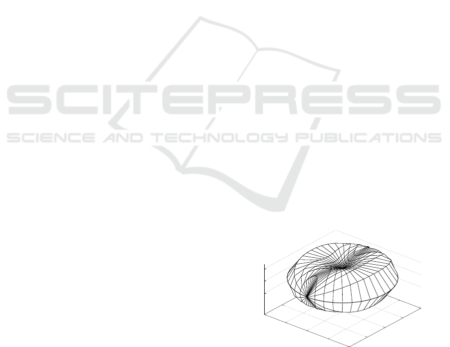
x
θ
y
-1
-0.5
0
0.5
1
-1
-0.5
0
0.5
1
-0.1
0
0.1
Figure 1: A nonholonomic sphere of the unicycle.
In Fig. 1 a nonholonomic sphere of the unicycle is
illustrated with the identity output function k
k
k(q
q
q) = q
q
q
and controls with full harmonics up to degree one in
Small Radius Spheres in Output Space of Nonholonomic Systems
319

both controls
(
u
1
(t) = p
1
1
+ p
2
1
sin(ωt) + p
3
1
cos(ωt),
u
2
(t) = p
1
2
+ p
2
2
sin(ωt) + p
3
2
cos(ωt).
(21)
A regular mesh used to describe possible directions of
motions is given as follows
(α
1
,α
2
) = (
πi
18
,
πj
18
), i= 0,1,..., 35; j = 0,1,...,18.
The sphere is radially symmetric with respect to the
y axis and the pure motion along the y-axis is least
energy-efficient.
For a given selection of α
α
α = (α
1
,α
2
)
T
an elemen-
tary optimization task has been solved to get the vec-
tor p
p
p realizing the maximum value of the distance R.
Next, the value of p
p
p was substituted into Eq. (21) to
determine controls and a numerical integration of the
model (18) initialized atq
q
q
0
with the controlsu
u
u was in-
voked. The final point of the trajectory generated con-
tributed into a numerically obtained nonholonomic
sphere visualized in Fig. 2. This sphere is a close ap-
proximation of the real nonholonomic sphere for the
unicycle. Both spheres are interlaced in Fig. 3.
x
θ
y
-1
-0.5
0
0.5
1
-1
-0.5
0
0.5
1
-0.2
0
0.2
Figure 2: A nonholonomic sphere of the unicycle obtained
with a numerical integration.
It can be observed that the spheres differ slightly
as the sphere obtained with the algorithm and based
on the gCBHD formula neglects the higher degree
vector fields while the numerical procedure takes
them into account implicitly. Nevertheless, the dif-
ference is small enough to plan a motion with the al-
gorithm in a desired direction.
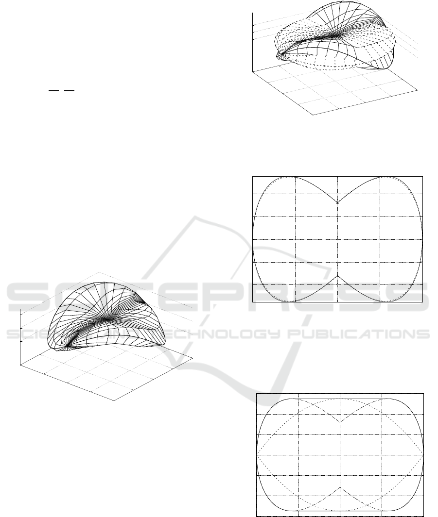
In Fig. 4 a section of spheres from Fig. 3 for
θ = 0 (the x − y plain) is presented. The solid line
corresponds to the sphere generated by the algorithm
while the dashed line – to a numerical integration of
the model. At this sections the differences are really
small. From the figure one can learn also that the mo-
tion along the second degree vector field [X
X
X,Y
Y
Y] acting
x
θ
y
-1
-0.5
0
0.5
1
-1
-0.5
0
0.5
1
-0.1
0
0.1
Figure 3: Nonholonomic spheres of the unicycle obtained
with the algorithm presented (dashed) and the numerical in-
tegration.
-0.1
-0.05
0
0.05
0.1
-1 -0.5 0 0.5 1
x
y
Figure 4: The section of nonholonomic spheres of the uni-
cycle for θ = 0.
at q
q
q
0
along y-axis is significantly less effective than a
motion along x-axis corresponding to the first degree
vector field X
X
X.
-0.15
-0.1
-0.05
0
0.05
0.1
0.15
-1 -0.5 0 0.5 1
x
y
Figure 5: The unicycle with a projection onto x − y plane
output function. The section for θ = 0 and three selections
of controls.
Now an impact of representation of controls and
output functions on sections of nonholonomicspheres
for the unicycle robot are investigated. In Fig. 5 and
ICINCO 2019 - 16th International Conference on Informatics in Control, Automation and Robotics
320

-0.15
-0.1
-0.05
0
0.05
0.1
0.15
-1 -0.5 0 0.5 1
x
y
Figure 6: The unicycle with the identity output function.
The section for θ = 0 and three selections of controls (the
solid line coincides with the dot-dashed one).
Fig. 6 three sections are presented for the output func-
tion k(q
q
q) = (x, y)
T
and k(q
q
q) = (x,y, θ)
T
, respectively:
solid line corresponds to controls given in Eq. (21),
the dashed line was obtained within the family of con-
trols
(
u
1
(t) = p
1
1
+ p
2
1
sin(ωt),
u
2
(t) = p
1
2
+ p
3
2
cos(ωt).
(22)
while the dot-dashed line corresponds to the controls
(
u
1
(t) = p
1
1
+ p
3
1
cos(ωt),
u
2
(t) = p
1
2
+ p
2
2
sin(ωt).
(23)
In all cases the algorithm presented in this paper has
generated the required data. From Figs. 5. 6, it can be
deduced that the representation of controls is very im-
portant as spheres (and their sections) generated can
differ in shapes significantly. Even when the repre-
sentation is of the same length (as in Eq. (22) and (23)
still the differences are visible). In practical situations
one should solve the following problem: how to get
reliable results keeping a representation of controls as
small as possible (as it significantly decreases compu-
tational costs).
For a kinematic car the output function is selected
as the identity k
k
k(q
q
q) = q
q
q and controls are full harmon-
ics up to the order of two
(
u
1
(t) = p
1
1
+
∑
2
j=1
(p
2j
1
sin( jωt) + p
2j+1
1
cos( jωt)),
u
2
(t) = p
1
2
+
∑
2
j=1
(p
2j
2
sin( jωt) + p
2j+1
2
cos( jωt)).
(24)
An irregular mesh of 47 points discretizing the α
1
angle and 43 points for the α
2
angle are selected to
discretize the space of α
α
α angles. The purpose to use
the irregular mesh instead of regular one is to keep
the computational complexity as low as possible with-
out deteriorating the quality of retrieving a shape of
spheres. While using a regular mesh, the vast major-
ity of points are located in the area close to planes
x
θ
y
-1
-0.5
0
0.5
1
-0.1
-0.05
0
0.05
0.1
-0.01
0
0.01
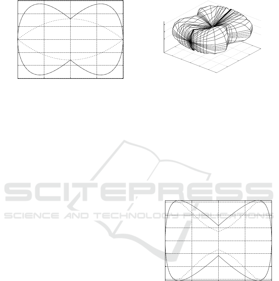
Figure 7: A section of the nonholonomic sphere of the kine-
matic car obtained with the algorithm for ψ = 0.
x = 0 or θ = 0. In Fig. 7 a section of the nonholo-
nomic sphere for the kinematic car calculated with the
algorithm is presented when ψ = 0. In Fig. 8 sections
of the sphere of the kinematic car are presented for
(θ = ψ = 0) (on the x− y plane). As before, the solid
curve is generated with the algorithm while dashed
one with a numerical integration of the model (19).
The section shapes presented in Fig. 8 are similar, but
with different values near the y axis. It is noticeable
a large difference between the maximal values of x
and y coordinates of points along the curves as the
vector field acting along x and y axis are of different
degrees.
-0.015
-0.01
-0.005
0
0.005
0.01
0.015
-1 -0.5 0 0.5 1
x
y
Figure 8: A section of the nonholonomic sphere of the kine-
matic car obtained with the algorithm for θ = ψ = 0.
Programs used in simulations were written in Wol-
fram Mathematica, version 11.3, (Wolfram Research,
2018) and run on a computer with Intel
R
 Core
TM
i5-8400 CPU and 8 GiB RAM memory. The com-
putational time to construct a sphere for the unicy-
cle was 210[s] and 36 × 19 elementary tasks (a di-
rectional optimization in a particular direction deter-
mined by fixing angles (α
1
,α
2
)) were solved which
gives 0.3[s]/task. The total computational time to
construct a kinematic car sphere’s section (ψ = 0) was
390[min] and 47 × 43 elementary tasks were solved
Small Radius Spheres in Output Space of Nonholonomic Systems
321

which gives 11.5[s]/task.
It should be pointed out that the
NMinimize func-
tion was used extensively to solve elementary tasks.
The function tries to find the global optimum and it is
time consuming. In real applications some dedicated
procedures should be implemented to reduce compu-
tational costs, form example by taking into account
results of previous optimizations and incorporate a lo-
cal optimization (e.g. some variants of the Newton al-
gorithm, (Nakamura, 1991)) instead of the global one.
5 CONCLUSIONS
In this paper small radius spheres were examined for
nonholonomic systems considered with accompany-
ing output functions. The presented algorithm to de-
rive the spheres is based on the generalized Campbell-
Baker Hausdorff-Dynkin formula and locally, around
a given point in the configurations space, shrinks the
series generated with this formula to leave only the
small number of items required to preserve a small
time local controllability of the system. To derive a
reliable shape of the sphere a large number of opti-
mization tasks should be solved. It was shown how
to decrease the dimension of the tasks being solved
by one. The simulation results shown that the selec-
tion of a representation of controls is crucial in de-
riving reliable shapes of the spheres. The representa-
tion should be rich enough to get constructed spheres
reliable. Unfortunately, too long representations dra-
matically increase computational costs as many tasks
with a nonlinear quality function and nonlinear con-
straints should be solved. Results of the paper can be
used directly in motion planning algorithms of non-
holonomic systems with an output function. In the
algorithms, at a current configuration, only one opti-
mization task is to be solved, thus computational costs
are reasonably low.
ACKNOWLEDGEMENT
The first author was supported by the Young Re-
searchers’ Program under Grant No. 0402/0158/18
while the second author was supported by the WUST
statutory grant No. 0401/0022/18.
REFERENCES
Altafini, C. (2001). Some properties of the general n-trailer.
Int. Journal of Control, 74(4):409–424.
Bayle, B., Renaud, M., and Fourquet, J. (2003). Nonholo-
nomic mobile manipulators: Kinematics, velocities
and redundancies. J. Intell. Robot. Syst., 36(1):45–63.
Bertsekas, D. (1996). Constrained Optimization and La-
grange Multiplier Methods. Athena Scientific, Bel-
mont, Massachusetts.
Chow, W. (1939).
¨
Uber Systeme von linearen partiellen Dif-
ferentialgleichungen erster Ordnung. Mathematische
Annalen, 117(1):98–105.
Duleba, I. (1998). Algorithms of Motion Planning for Non-
holonomic Robots. WUST Publ. House, Wroclaw.
Duleba, I. (2018). Kinematic models of doubly generalized
n-trailer systems. Journal of Intelligent and Robotic
Systems, pages 1–8. on-line.
Duleba, I. and Khefifi, W. (2006). Pre-control form of the
gcbhd formula for affine nonholonomic systems. Sys-
tems and Control Letters, 55(2):146–157.
Duleba, I. and Mielczarek, A. (2018). Controllability of
driftless nonholonomic systems in a task-space. In
Tchon, K. and Zielinski, C., editors, Advances in
Robotics, pages 311–318, Publ. House of the Warsaw
Univ. of Technology. in Polish.
Jakubiak, J., Tchon, K., and Magiera, W. J. (2010). Motion
planning in velocity affine mechanical systems. Inter-
national Journal of Control, 83(9):1965–1974.
Jean, F. (2014). Control of Nonholonomic Systems:
from Sub-Riemannian Geometry to Motion Planning.
SpringerBriefs in Mathematics. Springer.
LaValle, S. (2006). Planning Algorithms. Cambridge Uni-
versity Press.
Mielczarek, A. and Duleba, I. (2018). Theoretical and algo-
rithmic aspects of generating pre-control form of the
gcbhd formula. In 23nd Int. Conf. on Methods and
Models in Automation and Robotics, pages 905–909,
Miedzyzdroje, Poland.
Nakamura, Y. (1991). Advanced Robotics: Redundancy and
Optimization. Addison-Wesley.
Nakamura, Y., Chung, W., and Sordalen, O. (2001). Design
and control of the nonholonomic manipulator. IEEE
Trans. Robot. Autom., 17(1):48–59.
Spivak, M. (1999). A comprehensive introduction to differ-
ential geometry. Publ or Perish Inc., Houstron, Tx.,
3rd edition.
Strichartz, R. (1987). The Campbell-Baker-Hausdorff-
Dynkin formula and solutions of differential equa-
tions. Journ. of Functional Analysis, 72:320–345.
Vafa, Z. and Dubowsky, S. (1990). The kinematics and dy-
namics of space manipulators: the virtual manipulator
approach. Int. J. Robot. Research, 9(4):3–21.
Wolfram Research, I. (2018). Mathematica, Version 11.3.
Champaign, IL, 2018.
ICINCO 2019 - 16th International Conference on Informatics in Control, Automation and Robotics
322