Environment-aware Sensor Fusion using Deep Learning
Caio Fischer Silva
1,2 a
, Paulo V. K. Borges
1 b
and Jos
´
e E. C. Castanho
2 c
1
Robotics and Autonomous Systems Group, CSIRO, Australia
2
School of Engineering, S
˜
ao Paulo State University - UNESP, Bauru, SP, Brazil
Keywords:
Environment-aware Sensor Fusion using Deep Learning.
Abstract:
A reliable perception pipeline is crucial to the operation of a safe and efficient autonomous vehicle. Fusing
information from multiple sensors has become a common practice to increase robustness, given that different
types of sensors have distinct sensing characteristics. Further, sensors can present diverse performance
according to the operating environment. Most systems rely on a rigid sensor fusion strategy which considers
the sensors input only (e.g., signal and corresponding covariances), without incorporating the influence of the
environment, which often causes poor performance in mixed scenarios. In our approach, we have adjusted
the sensor fusion strategy according to a classification of the scene around the vehicle. A convolutional
neural network was employed to classify the environment, and this classification is used to select the best
sensor configuration accordingly. We present experiments with a full-size autonomous vehicle operating in
a heterogeneous environment. The results illustrate the applicability of the method with enhanced odometry
estimation when compared to a rigid sensor fusion scheme.
1 INTRODUCTION
With the recent advances in robotics, autonomous mo-
bile robots are now operating in a broad range of do-
mains. Some well-known examples include industrial
plants (Borges et al., 2013), urban traffic (Bojarski
et al., 2016) and agriculture (Lottes et al., 2018). The
navigation system required to perform efficiently in
such scenarios needs to be robust to several opera-
tional challenges such as obstacle avoidance and re-
liable localization. When the same vehicle/platform
navigates through significantly different environments,
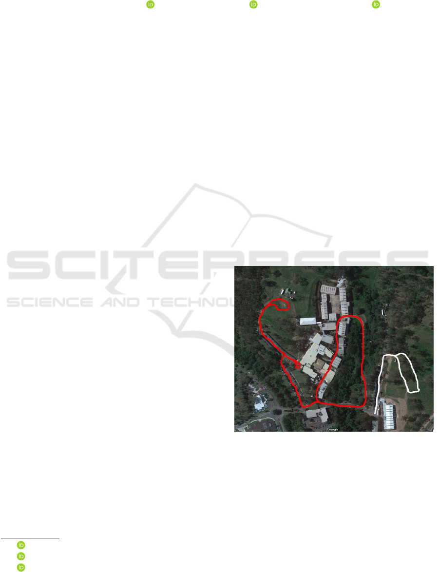
the navigation can be even more challenging. The
site shown in Figure 1 is representative of this situ-
ation. The highlighted paths represent sections on
which an autonomous vehicle should navigate to per-
form a given task. The image shows that different
regions of the tracks present distinct structural char-
acteristics. In some segments the vehicle must travel
through a densely built-up area, with large structures
and metallic sheds. In contrast, in other sections, the
path is unstructured and mostly surrounded by vegeta-
tion, including off-road terrain.
Sensors are required in robotic navigation to obtain
a
https://orcid.org/0000-0001-7948-5036
b
https://orcid.org/0000-0001-8137-7245
c
https://orcid.org/0000-0003-1762-7478
Figure 1: Satellite view illustrating a heterogeneous oper-
ation space. The red path were used to train the CNN to
classify the environment, while the white was used to vali-
date its performance. Image from Google Maps.
information about the robot’s surroundings. Since
each sensor has advantages and drawbacks, a single
sensor is often not sufficient to reliably represent the
world, and hence fusing data from multiple sensors has
become a common practice. Probabilistic techniques,
such as the Kalman filter (Maybeck, 1990a) and the
Particle filter (Maybeck, 1990b), enable sensor fusion
by explicitly modeling the uncertainty of each sensor.
88
Silva, C., Borges, P. and Castanho, J.
Environment-aware Sensor Fusion using Deep Learning.
DOI: 10.5220/0007841900880096
In Proceedings of the 16th International Conference on Informatics in Control, Automation and Robotics (ICINCO 2019), pages 88-96
ISBN: 978-989-758-380-3
Copyright
c
2019 by SCITEPRESS – Science and Technology Publications, Lda. All rights reserved
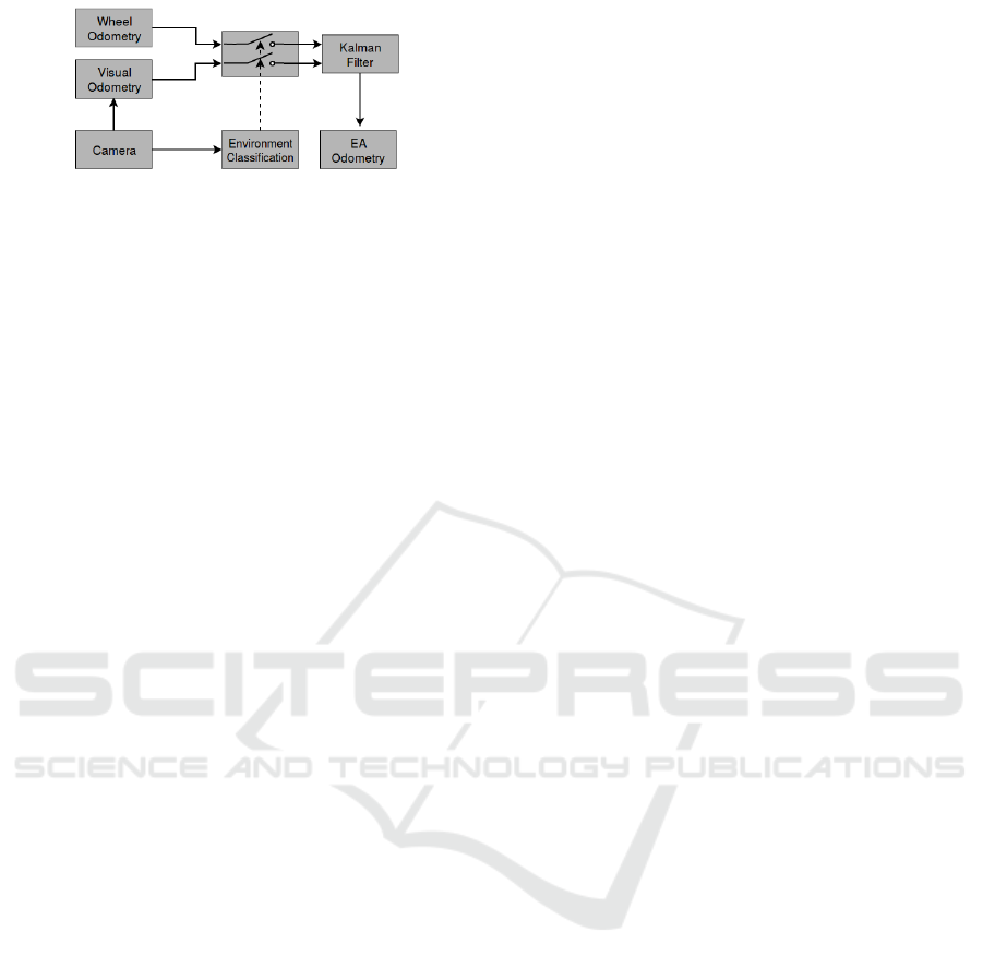
Figure 2: Architecture overview of the Environment-Aware
sensor fusion applied in odometry.
These are well-known approaches with optimal
performance when the navigation takes place in quite
homogeneous environments. However, in challenging
and mixed scenarios, as described above, employing
rigid statistical models of sensor noise may provide
a suboptimal solution. An environment-aware sensor
fusion, which dynamically adapts to each different
environment, can allow a better sensor fusion perfor-
mance.
Previous work using teach and repeat approach
illustrated the effectiveness of such adaptive scheme
(Rechy Romero et al., 2016), but it is limited to a pre-
viously defined path. To overcome this constraint, we
propose applying convolutional neural networks and
camera images to recognize typical navigation envi-
ronments (such as indoor, off-road, industrial, urban)
and associate that information to the best sensor-fusion
strategy. This approach is the gist of the method pro-
posed in this paper.
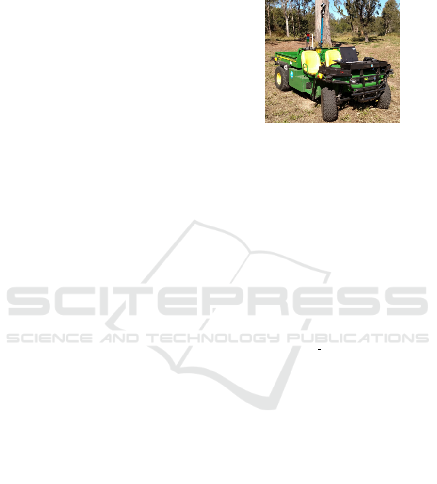
The proposed method was implemented and evalu-
ated in full-size autonomous utility vehicle developed
by the Robotics and Autonomous System Laboratory
at CSIRO, see Figure 4.
To validate the performance of the adaptive sensor
fusion scheme, we employed it to odometry estima-
tion. In the presence of ground truth, provided by a
reliable localization system, the error estimation in
odometry becomes trivial, which makes the perfor-
mance evaluation of the proposed method accurate
and straightforward.
Figure 2 shows a block diagram of the proposed
method. Experimental results have shown a reduction
in the estimation errors in comparison to using a rigid
combination of the sensors.
1.1 Related Work
Dividing the navigation map to consider different do-
mains has been used earlier to enhance the perfor-
mance of mobile robots (Lowry et al., 2016; Churchill
and Newman, 2012; McManus et al., 2012; Rechy
Romero et al., 2016). In this paradigm, usually known
as the teach and repeat, the navigation map is visited
in an initial phase in which the environment is learned.
Then, it is divided into sub-maps which are used later
to adjust the behavior of the robot. This paradigm was
employed in Furgale and Barfoot (2010), to enhance
navigation of long-range, autonomous operation of a
mobile robot in outdoor, GPS denied, and unstructured
environments. However, using sub-maps to change
system response can only be used in locations previ-
ously visited. That is, the behavior of the system is not
defined in unknown places, even if they are similar to
those visited before.
In Rechy Romero et al. (2016), an adaptive sen-
sor fusion technique is applied for obstacle detection.
It performs better than using each sensor alone or a
covariance-based weighted combination of them. The
authors have driven an automated vehicle through
a heterogeneous operation environment and quanti-
fied the performance of each obstacle-detecting sensor
along the trajectory. This information was used by
an environment-aware sensor fusion (EASF) strategy
that provides different confidence levels to each sensor
based on its location along the path. The method uses
a look-up table that relates the vehicle’s position with
the best sensor configuration.
In Suger et al. (2016), also proposed the use of
an adaptive approach to obstacle detection for mo-
bile robots. A random forest classifier was trained
to identify each environment using local geometrical
descriptors from a point cloud so it can classify places
not visited during the training. The work presents a
classification metric but does not elaborate on how the
adaptive strategy improved obstacle detection.
An adaptive scheme for robot localization was used
by Guilherme et al. (2016). The robot is equipped with
a short-range laser scanner and a Global Positioning
System (GPS) module. A histogram of the distances
between occupied cells on an occupancy grid from
the laser scanner was used to classify the environment
in outdoor or indoor using the k-nearest neighbor al-
gorithm. In outdoor environments, the localization
system would rely only on the GPS module, while
it uses the laser scanner and a previously built map
indoors.
In 2016, NVIDIA’s researchers (Bojarski et al.,
2016) have trained a convolutional neural network to
map the raw pixels from a front-facing camera to steer-
ing angles to control a self-driving car on roads and
highways (with or without lane markings). Accord-
ing to the authors, end-to-end learning leads to better
performance than optimizing human-selected interme-
diate criteria, like lane detection. This work has shown
the potential of convolutional neural networks to face
the highly challenging tasks of autonomous driving.
Zhou et al. (2014) have demonstrated that a properly
trained convolutional neural network can identify dif-
Environment-aware Sensor Fusion using Deep Learning
89
ferent environments based only on visual information,
using the so-called “deep features”.
These related works have shown that adding infor-
mation about the environment can lead to more robust
systems, able to operate on mixed scenarios. We com-
bine the teach and repeat paradigm with deep learning
based visual scene classification to optimize the sensor
fusion performance. As a result, our system assigns
the optimal sensor configuration to each scene based
only on visual information.
1.2 Visual Pose Estimation
Visual Odometry (VO) is the process of estimating the
movement of a robot given a sequence of images from
a camera attached to it. The idea was first introduced in
1980 for planetary rovers operating on Mars (Moravec,
1980).
However, it still a active research topic, as can be
seen from the fact that the work on visual odometry by
Forster et al. (2017) won the IEEE RAS Publication
Award in 2018.
The classical approach to VO relies on extracting
and tracking visual features, and then combine the
relative motion of these features in a sequence of im-
ages to estimate the camera’s movement. The process
of simultaneously localize the robot and map the en-
vironment using visual information is called Visual
SLAM.
The output of a VO system is usually fused with
other sensor modalities to improve its accuracy. A
popular choice for ground vehicles is fusing it with
wheel odometry (Bischoff et al., 2012), but inertial
sensors are broadly used as well (Corke et al., 2007).
2 ENVIRONMENT-AWARE
SENSOR FUSION
In this section we describe the framework for adaptive
sensor fusion, exploiting visual information from the
environment. We also provide a performance metric
used to compare each odometry method employed
and to define the best sensor configuration to each
environment.
2.1 Performance Metric
We chose the metric proposed by Burgard et al. (2009)
to compare the employed odometry methods. This
metric was proposed as an objective benchmark for
comparison of SLAM algorithms. Since it uses only
relative geometric relations between poses along the
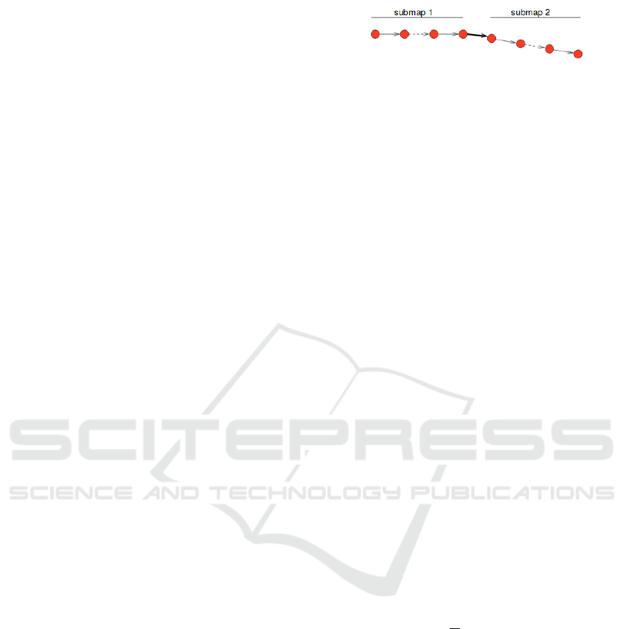
Figure 3: Example of why the absolute difference is subopti-
mal (Burgard et al., 2009).
robot’s trajectory, one can use it to compare odometry
methods without loss of generalization.
In the presence of a ground truth trajectory, it is
usual to get the odometry error by the absolute dif-
ference between the estimated poses and the ground
truth. Burgard et al. (2009) claim that this metric is
suboptimal because an error on the estimation of a sin-
gle transition between poses could increase the error
in all future poses. To illustrate this behavior, sup-
pose a robot moving in a straight line with a perfect
pose estimation system, but with a single rotation error
somewhere, let us say on the middle of the trajectory,
as shown on Figure 3.
Using the absolute difference would assign a zero
error to all the poses in the submap 1, as expected
considering an error-free pose estimator. But it would
assign a non-zero error to all the poses in the submap
2, even if the error is present only in the transition
between two particular poses, shown as a bold arrow
in the figure.
The proposed metric is based on the relative dis-
placement between the poses. Given two poses
x
i
and
x
j
in a trajectory,
δ
i, j
is defined as the relative transfor-
mation that moves from pose
x
i
to
x
j
. Given
x
1:T
, the
set of estimated poses, and
x
∗
1:T
, the ground truth ones.
The relative difference is defined in (1) as the squared
difference between the estimated and the ground truth
transformations, respectively
δ
and
δ
∗
. In the example
from Figure 3, the relative error is non-zero only for
the transformation represented by the bold arrow.
ε(δ) =
1
N
∑
i, j
(δ
i, j
δ
∗
i, j
)
2
(1)
By selecting the relative displacement
δ
i, j
, one can
highlight specific properties. For instance, by comput-
ing the relative displacement between nearby poses,
the local consistency is highlighted. In contrast, the
relative displacement between far away poses enforces
the overall geometry of the trajectory. In the experi-
ments, we used a mid-range displacement, big enough
to include some big scale geometry information while
highlighting local consistency.
We used a 10 seconds time interval to compute the
relative transformations, which resulted in a 25 meters
average distance between each pose when the vehicle
was moving in a straight line. The ground truth trajec-
tory was provided by a 3D LIDAR localization system,
ICINCO 2019 - 16th International Conference on Informatics in Control, Automation and Robotics
90
based on the SLAM algorithm proposed by Bosse and
Zlot (2009) operating in a previously mapped area.
2.2 Informed Sensor Fusion Strategy
We define a sensor configuration
λ
as the combination
of weights describing the reliability of each sensor.
Considering a system equipped with
n
different sen-
sors, the sensor configuration would be a vector of
n
elements as follows.
λ = [α
1
, α
2
, ..., α
n
]
T
∈ R
n
, with α
i
∈ [0, 1] (2)
Where
α
i
represents the reliability of the sensor
i
.
If it is equal to zero the sensor will not be used in the
fusion and if its value is one the sensor will be fused
using the provided error model. Intermediate values
should proportionally increase the uncertainty of the
sensor.
Appropriately changing the sensor configuration
can prevent the hazardous situation where the system
is very confident about a wrong estimation or the sub-
optimal situation where the system defines an unre-
alistic high uncertainty to a sensor in all scenarios to
compensate for its high error in some domains.
As described in Section 1.1, the teach and repeat
paradigm can be used to select a suitable sensor config-
uration, but in this work, we propose the use of visual
scene classification.
3 EXPERIMENTAL SET-UP
In this section, we describe the experimental set-up
and some implemented methods.
3.1 Vehicle Description
The robot is built upon a John Deere Gator, an electric
medium-size utility vehicle (see Figure 4). The vehi-
cle has been fully automated in the Robotics and Au-
tonomous System Laboratory at CSIRO (Egger et al.,
2018; Pfrunder et al., 2017).
The vehicle is equipped with a Velodyne VLP-16
Puck LIDAR, that provides a 360 degrees 3D point
cloud with a typical range accuracy of
±3cm
, which is
used for localization and obstacle avoidance. Besides
that, the vehicle has four safety 2D LIDARs (one on
each corner). Anytime an object is detected by the
lasers inside a safety zone an emergency stop signal is
triggered.
As usual in wheeled robots, the Gator has a wheel
odometer, made of a metal disc pressed onto the brake
drum and an inductive sensor. In addition to that, a
Figure 4: The robot used, a John Deere Gator holding multi-
ple sensors.
visual odometry algorithm was implemented using as
input images from an Intel RealSense D435 (Keselman
et al., 2017) mounted front facing in the vehicle, details
are provided in Section 3.2.
The vehicle holds two computers, one of them used
for the low-level hardware control and the other for
high-level tasks, such as localization and path planning.
The integration between the computers and the sensors
is done using the Robotics Operating System (ROS)
(Quigley et al., 2009).
3.2 Visual Odometry
A popular Visual SLAM implementation is the
ORB SLAM2 (Mur-Artal and Tard
´
os, 2017), which
uses the ORB (Oriented FAST and Rotated BRIEF)
feature detector. ORB SLAM2 is an open-source li-
brary for Monocular, Stereo and RGB-D cameras that
includes loop closure and relocalization capabilities.
We disabled the loop closure and relocalization treads
to get a pure visual odometry behavior.
The ORB SLAM2 classifies the detected features
into close and far key points applying a distance thresh-
old. The closest key points can be safely triangulated
between consecutive frames, providing a reliable trans-
lation inference. On the other hand, the farthest points
tend to give a more accurate rotation inference, since
multiple views support them.
Although the authors of ORB SLAM2 provide a
ROS node implementation, it is only able to read im-
ages from a ROS topic and output the final path as a
text file. We modified the library to provide a ROS
friendly interface, outputting the estimated position
and covariance in real-time, both in a ROS topic and
TF tree.
In addition to a standard RGB sensor, the Intel
RealSense D435 presents a stereo pair of infrared (IR)
cameras and an IR pattern projector used for RGB-D
imaging. The pair of IR images were used for the
visual odometry since it performed better than the
Environment-aware Sensor Fusion using Deep Learning
91

Figure 5: Sample image after the Adaptive Histogram Equal-
ization, the green dots stands for the detected ORB features.
RGB-D sensor while outdoors.
The images were equalized before the feature ex-
traction. The histogram equalization is a widespread
technique in image processing, used to enhance the
image’s contrast. It often performs poorly when the
image has a bi-modal histogram, images that have both
dark and bright areas. This effect was minimized using
the Contrast Limited Adaptive Histogram Equalization
(CLAHE) algorithm (Pizer et al., 1987).
Enhancing the contrast made it easier to find the
visual features, making the system more robust to chal-
lenging light conditions, inherent of the outdoor op-
eration. Figure 5 shows an image after the CLAHE,
with green dots indicating the extracted ORB features.
The features spread over the image, with some key
points close to the camera, enhancing the translation
estimation.
A demo video of the visual odometry running on
the Gator vehicle is available.
1
3.3 ROS robot localization Package
The Extended Kalman Filter (EKF) (Julier and
Uhlmann, 2004) is probably the most popular algo-
rithm for sensor fusion in robotics. Fusing wheel and
image sensors is a classic combination for odometry
(Bischoff et al., 2012), but there are other options,
such as Inertial Measurement Unit (IMU), LIDAR,
RADAR, and Global Positioning System (GPS).
The ROS package robot localization (Moore and
Stouch, 2014) provides an implementation of a non-
linear pose estimator (EKF) for robots moving in 3D
space. The package can fuse an arbitrary number of
sensors. It gets as parameter a binary vector indicating
which sensor should be fused and which one should be
ignored. This vector can be seen as a particular case
of sensor configuration as defined in Section 2.2.
1
https://youtu.be/I2bq0zsCuME
4 VISUAL ENVIRONMENT
CLASSIFICATION
The environment classification was treated as a classi-
cal supervised image classification problem. The oper-
ation area is shown in Figure 1 was divided into three
classes named industrial, parking lot and off-road.
In Section 2.2 we defined the sensor configuration
for informed sensor fusion, the reliability of each sen-
sor is a value between zero and one. Without loss of
generality, in our implementation we used the values
α
i
in Equation 2 as either zero or one, in a binary
representation.
In the industrial and the parking lot, the surface is
even, made of asphalt or concrete. In this scenario the
wheel slippage is low, and the wheel odometry presents
a low error. Even if the ground does not present many
visual features, the visual odometry performs properly
relying on the far key points. Hence, both sensors are
fused to estimate the odometry.
On the other hand, in the off-road environment,
the flatness assumption of human-made environments
does not hold, which allied with the increase in the
wheel slippage results in poor performance of the
wheel odometry. In contrast, the visual odometry can
benefit from the feature richness of the uneven terrain.
So, only the VO is used in this scenario.
The industrial and the parking lot classes could be
treated as a single class since both of then produces the
same sensor fusion behavior. We decided to keep both
classes instead of merging them since other parameters
could be changed according to these environments
on future works, like allowing reverse driving in the
parking lot.
We divided campus in two closed loops, the first
one used to collect the image to train the CNN and one
to validate the neural network’s classification perfor-
mance, respectively the red and white paths on Figure
1. Both paths present segments on the three classes, but
the second path was not exposed to the CNN during
the training phase.
Figure 6 shows samples of images used in the train-
ing and testing set. One can see the challenging light-
ing conditions, inherent of the outdoor operation.
A pre-trained implementation of the VGG16 (Si-
monyan and Zisserman, 2014) was used to classify the
images. The VGG16 is a 16-layer network used by
the VGG team in the ILSVRC-2014 competition. The
neural network was initially trained using
244 × 244
images assigned to one of the thousand labels present
in the Imagenet Dataset (Deng et al., 2009). By the
process of transfer learning, we froze the convolutional
layers to train our classifier using a custom built dataset
of the three classes described above.
ICINCO 2019 - 16th International Conference on Informatics in Control, Automation and Robotics
92

(a) (b) (c)
(d) (e) (f)
Figure 6: First row shows images used to train the CNN and
the second images used to validate the performance.
The transfer learning relies on the assumption that
the features learned to solve a particular problem on
computer vision might be useful to solve similar ones.
The main advantages of transfer learning are the reduc-
tion in training time and data requirements.
We used ten thousand images of each label. Since
the camera generates around thirty images per second,
it is not a demanding task to collect it. The images
were collected on different days and times of the day,
increasing the statistical significance of the dataset.
At the beginning of the training, the network strug-
gled in the transition between each scenario and some
segments on the off-road environment. By inspecting
the classification errors, looking for hard-negatives,
we detected that those were mostly pictures from the
off-road environment but showing buildings, cases that
the neural network misclassified as being an industrial
area. After collecting more data in this circumstance,
the neural network was able to yield a good general-
ization.
The classification using the neural network was
made at 15Hz on the same computer used to run the
visual odometry. Assuming that the environment does
not change at a high frequency, the real-time execu-
tion is not a requirement of the classifier. Thus the
prediction could be made less often to reduce the com-
putational burden.
5 EXPERIMENTS
We have defined two closed loops in the testing field.
Figure 1 shows path one in red and path two in white.
The path one was visited during the data collection
to train the classifier, as described in section 4. We
collected six and four samples from the path one and
two respectively.
The raw measurements of all the sensors were
saved during the data collection. After that, we esti-
Figure 7: Relative error in the second path.
mated offline the vehicle’s trajectory using each sensor
alone, a rigid fusion of the wheel and visual odome-
try and the environment-aware sensor fusion strategy
described before. These estimated trajectories were
compared with the ground truth poses to get the rela-
tive error as described in section 2.1.
6 RESULTS
6.1 Scene Classification Accuracy
After the data collection and the training described in
Section 4, the network achieved 98.7% classification
accuracy on the training set (red path) and 97.2% on
the validation set (white path). This high accuracy
might be seen as overfitting since both the training
and validation set were collected on the same cam-
pus. The accuracy in an extremely different landscape
would probably be much lower. However, that is also
a limitation on the teach and repeat approach.
By using convolutional neural networks, we pro-
vide the system with the ability to operate in places
never visited before. It should be noticed that the white
path, shown in Figure 1, was never visited during the
training phase.
Considering the high accuracy achieved on the net-
work validation, we expect a near optimum classifi-
cation and, as a consequence, the same sensor fusion
behavior on both paths.
6.2 Odometry Accuracy
Figure 7 shows the relative error for each odometry
method on a particular sample from second path. The
error in the wheel odometer is not on the plot to im-
prove the visualization since it is an order of magnitude
bigger. As expected, the error in the environment-
aware approach follows the trend of the approach with
the smaller error on each time interval.
The Tables 1 and 2 presents the average relative
error in the paths one and two respectively. Using only
the wheel odometry is the worst option on both. In
Environment-aware Sensor Fusion using Deep Learning
93

Table 1: Mean relative error in the training path.
Sensor Mean Relative Error (m)
Wheel Odometry 3.01(±0.57)
Visual Odometry (ORB SLAM2) 0.54(±0.09)
Wheel Odometry + Visual Odometry (EKF) 0.34(±0.10)
Environment-aware Sensor Fusion (EASF) 0.35(±0.10)
Table 2: Mean relative error in the testing path.
Sensor Mean Relative Error (m)
Wheel Odometry 2.72(±0.37)
Visual Odometry (ORB SLAM2) 0.49(±0.09)
Wheel Odometry + Visual Odometry (EKF) 0.65(±0.25)
Environment-aware Sensor Fusion 0.36(±0.10)
the red path, the EKF (rigid sensor fusion) improved
the odometry estimation in 57.2% when compared
with the visual odometry, while the EASF approach
improved only 55.4%. So the EASF was 1.8% less
accurate than the rigid sensor fusion scheme.
However, on the white path, the rigid fusion re-
sulted in a bigger error than using only the VO, proba-
bly due to the bad performance of the wheel odometry
on this scenario. This noise does not affect the EASF
scheme, that reduced the error by 31.1% regarding the
VO. So, the error in the EASF is more the 50% smaller
than the error in the EKF.
This difference in the average performance might
be caused by the low presence of the off-road scenario
in the first path. It is just a small section in a big
loop. On the other hand, the second path has near
equally distributed sections of both off-road and on-
road domains.
Since the covariance on the wheel odometry was
measured on the asphalt and concrete, it is not a good
representation of the error while driving off-road. This
overconfidence leads the rigid fusion to bad estima-
tions.
The results in the second path proved that using
the visual information to switch between odometry
sources according to the environment might lead to
a better performance than always fusing all available
sensors. In more challenging operational spaces, for
instance, paths including mud and gravel, our approach
might perform even better.
7 CONCLUSIONS
We have presented a new approach to dynamically
adapt a sensor fusion strategy for autonomous robot
navigation based on the surrounding environment.
Convolutional neural networks were trained to rec-
ognize images of the environment on which the robot
navigates and based on this information the system
adapts its sensor fusion strategy.
The proposed method can be seen as an extension
to the teach and repeat paradigm using convolutional
neural networks.
To validate the concepts, we also presented a prac-
tical implementation of the system on a full-size au-
tonomous vehicle. It is shown that, in environments
where the sensor behavior changes, it is possible to se-
lect a more suitable sensor configuration using visual
information to improve the odometry capabilities of
the system. Experimental results have shown an im-
provement in performance when compared to a rigid
sensor fusion approach.
On this project, the sensor configuration only in-
cludes binary values for the sensors reliability. We
expect that linearly changing the confidence level of
each sensor according to the environment would lead
to even better performance than our approach. One
way to vary the confidence level is by changing the
measurements covariances accordingly.
The results presented here only consider the use
of two sensors so future work could add more sen-
sors to the current framework. Another improvement
would be the implementation of an automatic label
scheme. It could be built using the performance met-
ric proposed in Section 2.1 to label each image with
the top performance sensor configuration. Further,
the methodology can also be extended to localization
and mapping, creating environment-aware mapping
strategies for long-term localization.
ACKNOWLEDGEMENTS
The authors would like to thank Russell Buchanan,
Jiadong Guo and the rest of the CSIRO team for their
assistance during this work. This work was partially
funded by the grant #2018/02122-0 Sao Paulo Reseach
ICINCO 2019 - 16th International Conference on Informatics in Control, Automation and Robotics
94

Foundation (FAPESP).
REFERENCES
Bischoff, B., Nguyen-Tuong, D., Streichert, F., Ewert, M.,
and Knoll, A. (2012). Fusing vision and odometry for
accurate indoor robot localization. In 2012 12th Inter-
national Conference on Control Automation Robotics
Vision (ICARCV), pages 347–352.
Bojarski, M., Testa, D. D., Dworakowski, D., Firner, B.,
Flepp, B., Goyal, P., Jackel, L. D., Monfort, M., Muller,
U., Zhang, J., Zhang, X., Zhao, J., and Zieba, K.
(2016). End to end learning for self-driving cars. arXiv
preprint arXiv:1604.07316.
Borges, P. V. K., Zlot, R., and Tews, A. (2013). Integrating
off-board cameras and vehicle on-board localization
for pedestrian safety. IEEE Transactions on Intelligent
Transportation Systems, 14(2):720–730.
Bosse, M. and Zlot, R. (2009). Continuous 3d scan-matching
with a spinning 2d laser. In 2009 IEEE International
Conference on Robotics and Automation, pages 4312–
4319.
Burgard, W., Stachniss, C., Grisetti, G., Steder, B.,
K
¨
ummerle, R., Dornhege, C., Ruhnke, M., Kleiner,
A., and Tard
´
os, J. D. (2009). Trajectory-based compar-
ison of slam algorithms. In In Proc. of the IEEE/RSJ
Int. Conf. on Intelligent Robots & Systems (IROS.
Churchill, W. and Newman, P. (2012). Practice makes per-
fect? managing and leveraging visual experiences for
lifelong navigation. In Robotics and Automation
(ICRA), 2012 IEEE International Conference on, pages
4525–4532. IEEE.
Corke, P., Lobo, J., and Dias, J. (2007). An introduction to
inertial and visual sensing. The International Journal
of Robotics Research, 26(6):519–535.
Deng, J., Dong, W., Socher, R., Li, L.-J., Li, K., and Fei-Fei,
L. (2009). Imagenet: A large-scale hierarchical image
database. In CVPR09.
Egger, P., Borges, P. V., Catt, G., Pfrunder, A., Siegwart,
R., and Dub
´
e, R. (2018). Posemap: Lifelong, multi-
environment 3d lidar localization. In 2018 IEEE/RSJ
International Conference on Intelligent Robots and
Systems (IROS), pages 3430–3437. IEEE.
Forster, C., Carlone, L., Dellaert, F., and Scaramuzza,
D. (2017). On-manifold preintegration for real-time
visual–inertial odometry. IEEE Transactions on
Robotics, 33(1):1–21.
Furgale, P. and Barfoot, T. D. (2010). Visual teach and
repeat for long-range rover autonomy. Journal of Field
Robotics, 27(5):534–560.
Guilherme, R., Marques, F., Lourenco, A., Mendonca, R.,
Santana, P., and Barata, J. (2016). Context-aware
switching between localisation methods for robust
robot navigation: A self-supervised learning approach.
In 2016 IEEE International Conference on Systems,
Man, and Cybernetics (SMC), pages 004356–004361.
IEEE.
Julier, S. J. and Uhlmann, J. K. (2004). Unscented filtering
and nonlinear estimation. Proceedings of the IEEE,
92(3):401–422.
Keselman, L., Iselin Woodfill, J., Grunnet-Jepsen, A., and
Bhowmik, A. (2017). Intel RealSense Stereoscopic
Depth Cameras. ArXiv e-prints.
Lottes, P., Behley, J., Milioto, A., and Stachniss, C. (2018).
Fully convolutional networks with sequential informa-
tion for robust crop and weed detection in precision
farming. IEEE Robotics and Automation Letters (RA-
L), 3:3097–3104.
Lowry, S., S
¨
underhauf, N., Newman, P., Leonard, J. J., Cox,
D., Corke, P., and Milford, M. J. (2016). Visual place
recognition: A survey. IEEE Transactions on Robotics,
32(1):1–19.
Maybeck, P. S. (1990a). The Kalman Filter: An Introduction
to Concepts. In Autonomous Robot Vehicles, pages
194–204. Springer New York, New York, NY.
Maybeck, P. S. (1990b). The Kalman Filter: An Introduction
to Concepts. In Autonomous Robot Vehicles, pages
194–204. Springer New York, New York, NY.
McManus, C., Furgale, P., Stenning, B., and Barfoot, T. D.
(2012). Visual teach and repeat using appearance-
based lidar. In 2012 IEEE International Conference
on Robotics and Automation, pages 389–396.
Moore, T. and Stouch, D. (2014). A generalized extended
kalman filter implementation for the robot operating
system. In Proceedings of the 13th International Con-
ference on Intelligent Autonomous Systems (IAS-13).
Springer.
Moravec, H. P. (1980). Obstacle Avoidance and Navi-
gation in the Real World by a Seeing Robot Rover.
PhD thesis, Stanford University, Stanford, CA, USA.
AAI8024717.
Mur-Artal, R. and Tard
´
os, J. D. (2017). Orb-slam2: An open-
source slam system for monocular, stereo, and rgb-d
cameras. IEEE Transactions on Robotics, 33(5):1255–
1262.
Pfrunder, A., Borges, P. V., Romero, A. R., Catt, G., and
Elfes, A. (2017). Real-time autonomous ground ve-
hicle navigation in heterogeneous environments using
a 3d lidar. In 2017 IEEE/RSJ International Confer-
ence on Intelligent Robots and Systems (IROS), pages
2601–2608. IEEE.
Pizer, S. M., Amburn, E. P., Austin, J. D., Cromartie, R.,
Geselowitz, A., Greer, T., ter Haar Romeny, B., Zim-
merman, J. B., and Zuiderveld, K. (1987). Adaptive
histogram equalization and its variations. Computer vi-
sion, graphics, and image processing, 39(3):355–368.
Quigley, M., Conley, K., Gerkey, B. P., Faust, J., Foote, T.,
Leibs, J., Wheeler, R., and Ng, A. Y. (2009). Ros:
an open-source robot operating system. In ICRA
Workshop on Open Source Software.
Rechy Romero, A., Koerich Borges, P. V., Elfes, A., and
Pfrunder, A. (2016). Environment-aware sensor fusion
for obstacle detection. In 2016 IEEE International
Conference on Multisensor Fusion and Integration for
Intelligent Systems (MFI), pages 114–121. IEEE.
Simonyan, K. and Zisserman, A. (2014). Very Deep Convo-
lutional Networks for Large-Scale Image Recognition.
arXiv e-prints, page arXiv:1409.1556.
Suger, B., Steder, B., and Burgard, W. (2016). Terrain-
adaptive obstacle detection. In 2016 IEEE/RSJ Inter-
Environment-aware Sensor Fusion using Deep Learning
95

national Conference on Intelligent Robots and Systems
(IROS), pages 3608–3613.
Zhou, B., Lapedriza, A., Xiao, J., Torralba, A., and Oliva, A.
(2014). Learning Deep Features for Scene Recognition
using Places Database.
ICINCO 2019 - 16th International Conference on Informatics in Control, Automation and Robotics
96
