Knowledge Transfer in a Pair of Uniformly Modelled Bayesian Filters

Ladislav Jirsa

, Lenka Kukli

sov

a Pavelkov

1 a

and Anthony Quinn

1,2 b

Institute of Information Theory and Automation, The Czech Academy of Sciences, Prague, Czech Republic

Trinity College Dublin, The University of Dublin, Ireland

Keywords:

Fully Probabilistic Design, Bayesian Filtering, Uniform Noise, Knowledge Transfer, Predictor, Orthotopic

Bounds.

Abstract:

The paper presents an optimal Bayesian transfer learning technique applied to a pair of linear state-space

processes driven by uniform state and observation noise processes. Contrary to conventional geometric ap-

proaches to boundedness in ﬁltering problems, a fully Bayesian solution is adopted. This provides an approxi-

mate uniform ﬁltering distribution and associated data predictor by processing the involved bounds via a local

uniform approximation. This Bayesian handling of boundedness provides the opportunity to achieve optimal

Bayesian knowledge transfer between bounded-error ﬁltering nodes. The paper reports excellent rejection of

knowledge below threshold, and positive transfer above threshold. In particular, an informal variant achieves

strong transfer in this latter regime, and the paper discusses the factors which may inﬂuence the strength of

this transfer.

1 INTRODUCTION

The problem of data (also known as measurement or

information) fusion is now key in many areas of in-

dustry, driven by the IoT and Industry 4.0 agendas

(Diez-Olivan et al., 2019). Data fusion systems are

required in areas such as sensor networks, robotics,

and video and image processing systems (Khaleghi

et al., 2013). Applications range from health moni-

toring (Vitola et al., 2017) and environmental sensing

(Zou et al., 2017), to cooperative systems for indoor

tracking (Dardari et al., 2015) or urban vehicular lo-

calization (Nassreddine et al., 2010). In all cases, in-

formation about the same quantity of interest (or sev-

eral quantities of interest, related in a speciﬁed way)

is acquired by different types of detectors, under dif-

ferent conditions, via multiple experiments and mea-

surement devices. (Lahat et al., 2015) provides an

overview of the main challenges in multimodal data

fusion across various disciplines, while the survey in

(Gravina et al., 2017) discusses clear motivations and

advantages of multi-sensor data fusion.

Diverse approaches to solving data fusion prob-

lems have been proposed in the literature, very of-

ten driven by the speciﬁcs of the application, and

it is clear that no universal deﬁnition—much less

https://orcid.org/0000-0001-5290-2389

https://orcid.org/0000-0002-3873-7556

a universal solution—has yet been accepted. Wiener-

type criteria for measurement vector fusion (Will-

ner et al., 1976) have long been available, while di-

rect variants of the Kalman ﬁlter have also been pro-

posed for fusion of measurements (Dou et al., 2016)

and states (Yang et al., 2019). Artiﬁcial intelligence

(Xiao, 2019), machine learning (Vitola et al., 2017;

Shamshirband et al., 2015; Vapnik and Izmailov,

2017) and expert system approaches (Majumder and

Pratihar, 2018) have all yielded progress in this area.

In the Bayesian framework which we adopt in this

paper, concepts of data, knowledge and information

are all uniﬁed via a probabilistic representation, being

typically the distribution of the unknown quantities of

interest, conditioned by data. Each measurement pro-

cess (node or sensor) constructs its local distribution

conditioned on its locally sensed data. The inferred

quantity may be globally shared by all the nodes, or

these may be distinct but related quantities (Azizi and

Quinn, 2018). The task is then one of optimal merg-

ing of these local distributions, a problem closely re-

lated to distributional pooling (Abbas, 2009). An-

other closely related problem is that of knowledge

transfer (Torrey and Shavlik, 2010). Again, in the

Bayesian context of this paper, the requirement is to

transfer probabilistic knowledge (a distribution) from

secondary (i.e. external or source) nodes to a pri-

mary node, to support its inference of the quantity

Jirsa, L., Pavelková, L. and Quinn, A.

Knowledge Transfer in a Pair of Uniformly Modelled Bayesian Filters.

DOI: 10.5220/0007854104990506

In Proceedings of the 16th International Conference on Informatics in Control, Automation and Robotics (ICINCO 2019), pages 499-506

ISBN: 978-989-758-380-3

499

of interest. Optimal Bayesian transfer learning via

Kullback-Leibler divergence (KLD) minimization—

known as fully probabilistic design (FPD) (Quinn

et al., 2016)—is developed in (Quinn et al., 2017),

and specialized to the case of data-predictive transfer

between Kalman ﬁlters in (Foley and Quinn, 2018),

(Pape

z and Quinn, 2018). In this approach, the sec-

ondary data predictor is transferred to the primary

ﬁltering node via an optimal mean-ﬁeld-type opera-

tor. This is shown to improve the primary state re-

construction in positive transfer cases, and rejects the

secondary knowledge otherwise. In addition to the

consistency and optimality properties of this Bayesian

transfer learning framework, a key practical advan-

tage here is that the relationship between the primary

and secondary processes does not have to be explicitly

modelled.

In this paper, we address the important prac-

tical context where the involved uncertainties are

bounded. Contemporary examples of sensor networks

with bounded innovations and/or observation pro-

cesses are studied in (Goudjil et al., 2017; He et al.,

2017; Vargas-Melendez et al., 2017). Speciﬁcally,

we extend the Bayesian transfer learning technique in

(Quinn et al., 2017) to a pair of linear state-space pro-

cesses driven by uniform state and observation noise

processes. Boundedness in ﬁltering problems is han-

dled via several approaches. Within the Kalman ﬁl-

tering set-up, the state estimates are projected onto

the constraint surface (Fletcher, 2000) or the Gaussian

distribution is truncated (Simon and Simon, 2010).

Using sequential Monte-Carlo sampling methods, the

constraints are respected within the accept/reject steps

of the algorithm, see e.g. (Lang et al., 2007). The

non-probabilistic techniques dealing with “unknown-

but-bounded error” provide an approximate set con-

taining the estimates (Chisci et al., 1996), (Becis-

Aubry et al., 2008). Recently, a fully Bayesian so-

lution has yielded a sequentially uniform ﬁltering dis-

tribution (Pavelkov

a and Jirsa, 2018) and associated

data predictor (Jirsa et al., 2019) by processing the

involved bounds via a local uniform approximation

of the state predictor at each ﬁltering step, achiev-

ing a recursive, tractable algorithm. This Bayesian

handling of boundedness now provides the opportu-

nity for optimal Bayesian knowledge transfer between

bounded-error ﬁltering nodes, as set out below.

Throughout the paper, z

is the value of a column

vector z at a discrete time instant t ∈ t

≡ {1, 2,...,t};

t;i

is the i-th entry of z

; z(t) ≡ {z

t−1

,. . . ,z

}; z

and z are lower and upper bounds on z, respectively;

≡ means equality by deﬁnition, ∝ means equality up

to a constant factor. The symbol f (·|·) denotes a con-

ditional probability density function (pdf); names of

arguments distinguish respective pdfs; no formal dis-

tinction is made between a random variable, its real-

isation and an argument of the pdf. U

(z,z) denotes

the uniform pdf of z with the orthotopic support [z, z].

Also, χ(x ∈ x

) is the indicator function, i.e. if x ∈ x

then χ(x ∈ x

) = 1, otherwise χ(x ∈ x

) = 0.

2 UNIFORMLY MODELLED

BAYESIAN FILTERS:

KNOWLEDGE

REPRESENTATION AND

TRANSFER

We consider a pair of Bayesian ﬁlters, and distinguish

between the primary ﬁlter (called the target node in

transfer learning (Torrey and Shavlik, 2010) and the

secondary ﬁlter (sometimes called the source node),

with all sequences and distributions subscripted by

“s” in the latter case. Each ﬁlter processes its local

observation sequence, y

and y

s,t

, t ∈ t

, respectively,

informative of their local, hidden (state) process, x

and x

s,t

, respectively.

In this paper, we adopt linear stochastic state-

space models with known parameters for all four pro-

cesses, each driven by an independent, uniformly-

distributed white noise process of known parameters.

We summarize (isolated) Bayesian ﬁltering for this

class of model in Section 2.1. We brieﬂy review prob-

abilistic knowledge transfer between a pair of general

Bayesian ﬁlters in Section 2.2, using the axiomati-

cally optimal FPD principle. Then, in Section 2.3,

we instantiate this FPD-optimal transfer in the current

context of uniformly driven Bayesian ﬁlters, recover-

ing a tractable, recursive ﬂow via a local uniform ap-

proximation at each step.

2.1 Bayesian Filtering with Uniformly

Distributed Noise Processes

In the considered Bayesian set up (K

arn

y et al., 2005),

the system is described by the following pdfs:

prior pdf: f (x

) (1)

observation model: f (y

)

time evolution model: f (x

t−1

)

where y

is a scalar observable output, u

is a known

system input (optional, for generality), and x

is an

`-dimensional unobservable system state, t ∈ t

We assume that (i) hidden process x

satisﬁes the

Markov property, (ii) no direct relationship between

input and output exists in the observation model,

ICINCO 2019 - 16th International Conference on Informatics in Control, Automation and Robotics

500

and (iii) the inputs consist of a known sequence

,. . . ,u

t−1

Bayesian sequential state estimation (known as

ﬁltering) consists of the evolution of the posterior

pdf f (x

|d(t)) where d(t) is a sequence of observed

data records d

= (y

), t ∈ t

. The evolution of

f (x

|d(t)) is described by a two-steps recursion that

starts from the prior pdf f (x

Time Update: f (x

|d(t − 1)) =

t−1

f (x

t−1

) f (x

t−1

|d(t − 1))dx

t−1

, (2)

Data Update: f (x

|d(t)) =

f (y

) f (x

|d(t − 1))

f (y

) f (x

|d(t − 1))dx

f (y

) f (x

|d(t − 1))

f (y

|d(t − 1))

(3)

We introduce a linear state space model with a uni-

form noise (LSU model) in the form

f (x

t−1

) = U

( ˜x

− ρ, ˜x

+ ρ)

f (y

) = U

( ˜y

− r, ˜y

+ r). (4)

where ˜x

= Ax

t−1

+ Bu

t−1

, ˜y

= Cx

, A, B, C are the

known model matrices/vectors of appropriate dimen-

sions, ν

∈ (−ρ, ρ) is the uniform state noise with

known parameter ρ, n

∈ (−r, r) is the uniform ob-

servation noise with known parameter r.

State estimation of LSU model (4) according to

(2) and (3) leads to a very complex form of poste-

rior pdf. In (Pavelkov

a and Jirsa, 2018)

, an approxi-

mate Bayesian state estimation of this model (based

on a minimising of Kullback-Leibler divergence of

two pdfs) is proposed. The presented algorithm pro-

vides the evolution of the approximate posterior pdf

f (x

|d(t)) that is uniformly distributed on a parallelo-

topic support.

Approximate Time Update. The time update starts

at the time t = 1 with f (x

t−1

|d(t − 1)) = f (x

) =

). Being χ the indicator function, it holds

f (x

|d(t − 1)) ≈

∏

i=1

χ(m

t;i

− ρ

≤ x

t;i

≤ m

t;i

+ ρ

)

t;i

− m

t;i

+ 2ρ

∏

i=1

t;i

− ρ

t;i

+ ρ

) = U

− ρ, m

+ ρ),

(5)

Note that the paper (Pavelkov

a and Jirsa, 2018) con-

tains the typo in the formula (3): the relevant integration

variable should be x

instead of x

t−1

where m

= [m

t;1

,. . . , m

t;`

]

, m

= [m

t;1

,. . . , m

t;`

]

t;i

∑

j=1

min(A

i j

t−1; j

+ B

t−1

i j

t−1; j

+ B

t−1

(6)

t;i

∑

j=1

max(A

i j

t−1; j

+ B

t−1

i j

t−1; j

+ B

t−1

i j

means the term on the i-th row and the j-th column

of A.

Approximate Data Update. According to (3), we

process the observation y

as y

−r ≤ Cx

≤ y

+r (see

(4)) by the Bayes rule together with the prior (5) from

the time update. The approximate posterior pdf is uni-

formly distributed on a parallelotopic support

f (x

|d(t)) ≈ K

χ(x

≤ M

≤ x

), (7)

where K

is a normalising constant.

However, the time update (5) in the next step as-

sumes pdf with an orthotopic support. Therefore, the

parallelotope x

≤ M

≤ x

in (7) is circumscribed by

an orthotope x

≤ x

. In this way, we obtain an

approximate “orthotopic” posterior pdf

f (x

|d(t)) ≈ U

, x

). (8)

The orthotopic bounds x

and x

are used in the next

time update step (5) for the computation of the terms

m and m (6) and for the computation of point esti-

mates of states ˆx

ˆx

+ x

. (9)

Predictive pdf for LSU Model. The data predic-

tor of a linear state-space model is the denominator

of (3), where f (y

) is given by (4) and f (x

|d(t −

1)) is the result of the approximate time update (5).

The approximate uniform predictor as proposed in

(Jirsa et al., 2019) is

f (y

|d(t − 1)) ≈



− y



−1



≤ y



, (10)

where

= Cs − r (11)

= Cs + r (12)

for s and s deﬁned so that

= m

t;i

− ρ

, s

= m

t;i

+ ρ

, if C

≥ 0,

= m

t;i

+ ρ

, s

= m

t;i

− ρ

, if C

< 0,

(13)

This predictive pdf is conditioned by m

and m

considered as statistics, provided the parameters A

and B be known.

Mean value ˆy

≡ E[y

|d(t − 1)] of (10) is

E[y

|d(t − 1)] =

+ y

= C



+ m



| {z }

E[x

|d(t−1)]

. (14)

Knowledge Transfer in a Pair of Uniformly Modelled Bayesian Filters

501

2.2 FPD-optimal Knowledge Transfer

between Bayesian Filters

If knowledge transfer from the secondary to the pri-

mary ﬁlter is to be effective (the case known as pos-

itive transfer (Torrey and Shavlik, 2010)), then we

must assume that y

(t) is informative of x(t). The core

technical problems to be addressed are (i) that there is

no complete model relating x(t) and x

(t), and, there-

fore, (ii) probability calculus (i.e. standard Bayesian

conditioning) does not prescribe the required primary

distribution conditioned on the transferred knowl-

edge. Note that standard Bayesian conditioning yields

the solution only in the case of complete modelling

(Karbalayghareh et al., 2018). However, an insistence

on speciﬁcation of a complete model of inter-ﬁlter de-

pendence may be highly restrictive, and incur model

sensitivity in applications.

Instead, we acknowledge that the required condi-

tional primary state predictor,

f (x

|d(t − 1), f

), after

transfer of the secondary data predictor, f

(t −

1)) (10), is non-unique. Therefore, we solve the in-

curred decision problem optimally via the fully prob-

abilistic design (FPD) principle (Quinn et al., 2016),

choosing between all cases of

f (x

|d(t − 1), f

) con-

sistent with the knowledge constraint introduced by

the transfer of f

(t − 1)) (Quinn et al., 2017).

FPD axiomatically prescribes an optimal choice, f

as a minimizer of the Kullback-Leibler divergence

(KLD) from

f to an ideal distribution, f

, chosen by

the designer (K

arn

y and Kroupa, 2012):

|d(t − 1), f

) ≡ arg

f ∈F

minD(

f || f

). (15)

Here, the KLD is deﬁned as

f || f

) = E

, (16)

and F denotes the set of

f constrained by f

(Quinn

et al., 2016),(Quinn et al., 2017). The ideal distribu-

tion is consistently deﬁned as

|d(t − 1)) ≡ f (x

|d(t − 1)),

being the state predictor of the isolated primary ﬁl-

ter (5) (i.e. in the absence of any transfer from a sec-

ondary ﬁlter). In (Foley and Quinn, 2018), the follow-

ing mean-ﬁeld operator was shown to satisfy (15), and

so to constitute the FPD-optimal primary state pre-

dictor after the (static) knowledge transfer speciﬁed

above:

|d(t − 1), f

) ∝ f (x

|d(t − 1)) ×

×exp





(t − 1))ln f (y

)dy





. (17)

Note that the optional input u

is known and con-

stant. Here, it is not a part of FPD and plays only the

role of a conditioning quantity in d(t − 1).

2.3 FPD-optimal Uniform Knowledge

Transfer

Here, we express the KLD minimiser (17) in the case

of uniform pdfs. The functions appearing in (17) are

f (x

|d(t − 1)) ∝ χ (m

− ρ ≤ x

≤ m

+ ρ) (18)

(t − 1)) ∝ χ



≤ y



(19)

f (y

) ∝ χ (Cx

− r ≤ y

≤ Cx

+ r), (20)

see (5), (10) and (4). Then, the form of (17) is

|d(t − 1), f

) ∝ χ(m

− ρ ≤ x

≤ m

+ ρ) ×

×exp







≤ y



×ln χ (Cx

− r ≤ y

≤ Cx

+ r) dy





(21)

The ﬁrst term in the integral indicates the integration

limits are y

and y

. The characteristic function in

the logarithm must equal one, which zeroes the expo-

nent and generates an additional constraint for x

Imposing y

∈ (Cx

− r,Cx

+ r) ∩ (y

) with

nonempty intersection, we get the constraint for x

− r ≤ Cx

≤ y

+ r. (22)

The constraining inequalities in (22) represent a strip

in the state space. Time update of the target ﬁlter

yields an orthotope domain in the state space (Fig-

ure 2). The strip, containing information from the

source ﬁlter, and the orthotope then intersect (left side

of Figure 2). This constrained set is the form of the

knowledge transfer between the ﬁlters.

However, the data update step requires the prior

pdf to be on the orthotope domain. Therefore, the

constrained set must be circumscribed by another or-

thotope. The orthotope is an intersection of ` per-

pendicular strips. According to (Vicino and Zappa,

1996), all the ` + 1 strips are tightened, i.e. shifted

and/or narrowed, so that distance of their planes is

minimal while their intersection is unchanged (re-

moved redundancy). Then, the tightened ortho-

tope is the domain of the approximate expression of

ICINCO 2019 - 16th International Conference on Informatics in Control, Automation and Robotics

502

|d(t −1), f

) as the constrained prior entering the

data update.

Note: The similarity of (22) with the observa-

tion model (4) and their similar processing indicates

similarity of the constraint step and the data update

step. The difference is that the knowledge trans-

fer (22) accepts the interval, i.e. the uniform distri-

bution U

), whereas the data update is sup-

plied with the observed point, y

. This point can be

interpreted as the Dirac distribution δ

(y − y

). In this

distributional sense, both the steps are equivalent.

2.4 Algorithmic Summary

The source and target ﬁlters run their state estimation

tasks in parallel. The source ﬁlter is run in isolation,

and the data predictor (10) is computed between the

time update and data update steps. Processing of the

source predictor is placed between time update and

data update step in the target ﬁlter.

Initialisation:

• Choose ﬁnal time t > 0, set initial time t = 0

• Set values x

, x

, u

, noises ρ, r, r

On-line:

1. Set t = t +1

2. Compute m

, m

according to (6) for each ﬁlter

3. Time update: compute (5) for each ﬁlter

4. Compute data predictor of the source ﬁlter (10)

5. Knowledge transfer: get the constraining strip

(22) from the source data predictor and process

it to time updated pdf of the target ﬁlter ((22)

and below) to transfer knowledge between the

ﬁlters (alternatively, use the informal transfer

described later)

6. Get new data u

, y

7. Data update: add the data strip (4) and approx-

imate the obtained support by a parallelotope

(for details see Appendix A.2 in (Pavelkov

a and

Jirsa, 2018)) to obtain the resulting form (7)

(alternatively, skip the parallelotope stage and

only tighten the strips, as described in 5.) for

each ﬁlter

8. Compute x

, x

(8) for each ﬁlter

9. Compute the point estimate ˆx

(9) for the target

ﬁlter

10. If t < t, go to 1.

3 EXPERIMENTS

In this section, the simulation experiments demon-

strate the proposed algorithm properties.

3.1 Experiment Setup

We simulate the system studied in (Foley and Quinn,

2018), x

∈ R

, y

∈ R. The known model parameters

are A =



1 1

0 1



, C = [1 0], ρ = 1

(2)

×10

−5

, where

(2)

is the unit vector of length 2, r = 10

−3

. B =





, u

= 0, i.e. a system without input/control.

The estimation was run for t = 50 time steps. We in-

vestigate the inﬂuence of the observation noise r

the source ﬁlter (20) on estimate precision of the tar-

get ﬁlter, quanitiﬁed by TNSE (total norm squared-

error) deﬁned as TNSE =

∑

t=1

k ˆx

− x

, where k · k

is the Euclidean norm. For each combination of the

parameters, the computation was run 2000-times and

the TNSEs were averaged.

Simulated states x

, together with the state noise

ρ, are common for both the source and target ﬁlters,

whereas the observation noises r and r

, contributing

to observed values, differ. This simple setup is sufﬁ-

cient for illustration of the described method.

3.2 Results

-8 -7 -6 -5 -4 -3 -2 -1

log

-5.26

-5.25

-5.24

-5.23

-5.22

-5.21

-5.2

-5.19

log

TNSE

FPD transfer, r = 0.001

knowledge transfer

isolated filter

Figure 1: TNSE of the target LSU ﬁlter as a function of

the observation noise variance r

of the source ﬁlter. FPD

transfer.

Figure 1 shows the inﬂuence of the source ﬁlter

observation noise r

on precision of the target ﬁlter

through the FPD knowledge transfer. The method re-

jects negative knowledge transfer (unlike in the Gaus-

sian transfer case (Foley and Quinn, 2018)). For

higher values of r

, estimate precision coincides with

the isolated target ﬁlter (despite ﬂuctuations) and does

not increase. However, decrease of estimation error

for smaller r

is not very signiﬁcant, compared to (Fo-

ley and Quinn, 2018).

Knowledge Transfer in a Pair of Uniformly Modelled Bayesian Filters

503

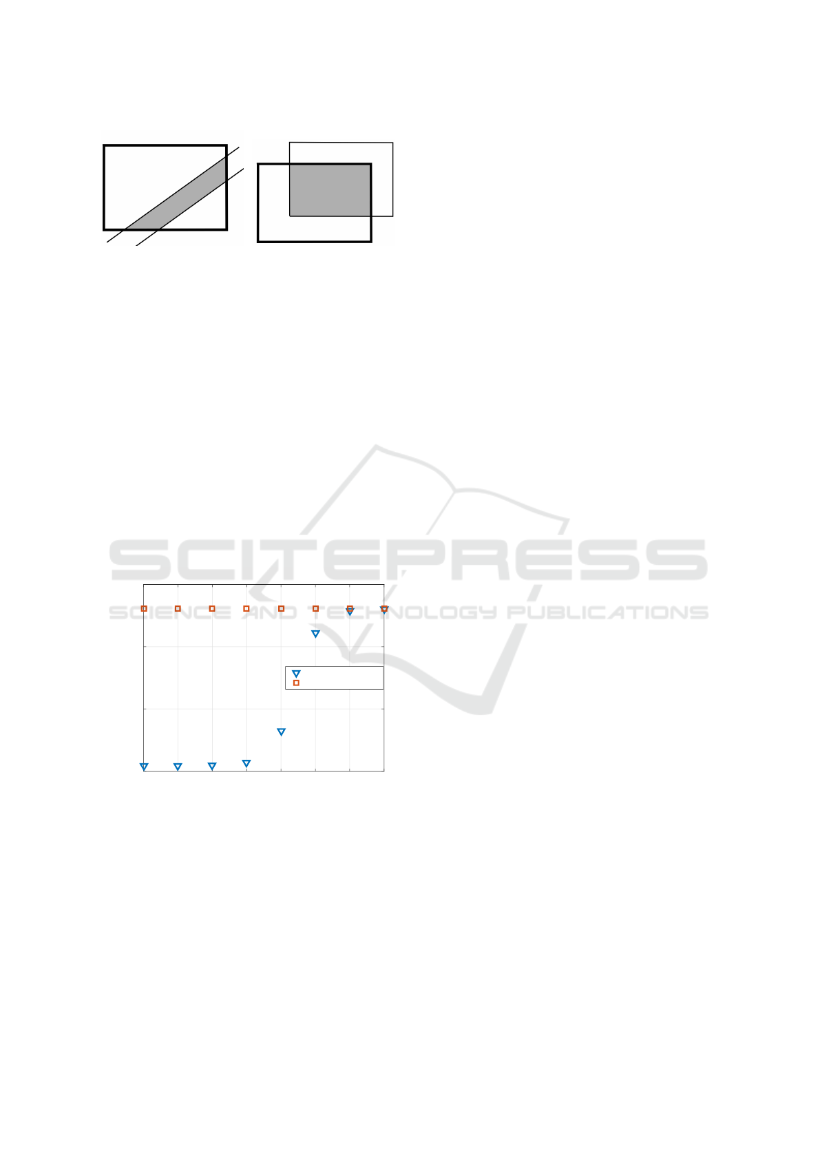
Figure 2: Domain of x

. Thick line: target ﬁlter, thin line:

transferred set. Left: FPD transfer. Right: informal transfer.

The probable reason for this last point can be il-

lustrated by the left part of Figure 2. The grey area

(the intersection) is to be circumscribed by an ortho-

tope (5). If the strip is too close to the diagonal, the

circumscribing orthotope is similar to the one given

by the time update (if the diagonal is contained in the

strip, the orthotopes are identical). This effect is prob-

ably caused by the fact that orthotopes are too conser-

vative as approximators.

The knowledge transfer acts as a constraint of the

target x

set by the source ﬁlter. This inspires an infor-

mal transfer, illustrated in the right part of Figure 2.

The idea is to use the intersection of the source and

target time-updated state sets. Although this approach

is not theoretically justiﬁed, it seems more suitable for

orthotopic sets. The results of the prediction errors

can be seen in Figure 3, in this informal case. The

-8 -7 -6 -5 -4 -3 -2 -1

log

-6.5

-6

-5.5

-5

log

TNSE

Informal transfer, r=0.001

knowledge transfer

isolated filter

Figure 3: TNSE of the target LSU ﬁlter as a function of the

observation noise variance r

of the source ﬁlter. Informal

transfer.

behaviour is qualitatively the same as in the previous

case, but the inﬂuence on the target ﬁlter precision

is now much more signiﬁcant in the positive transfer

regime.

It has also been observed that omitting the paral-

lelotope stage in the data update, i.e. involving only

strip tightening as in the FPD-based knowledge trans-

fer, makes no difference in the target state precision.

3.3 Discussion

The isolated LSU ﬁlter performance serves as a refer-

ence against which to assess the effect of the knowl-

edge transfer from a source LSU ﬁlter to a target one.

A key advantage of the FPD-transfer—apart from its

decision-theoretic optimality—is that the (stochastic)

relationship between the ﬁlters does not have to be

speciﬁed (in contrast to standard Bayesian transfer

learning techniques (Karbalayghareh et al., 2018)).

This confers robustness on the approach.

Both the FPD and informal transfers of Section 3

exhibit an important property: the ability to reject

the source knowledge in the “below-threshold” case

of inferior-quality data-predictive knowledge transfer

(i.e. where r

≥ r). This form of robustness is in con-

trast to FPD transfer between Kalman ﬁlters (Gaus-

sian transfer) reported in (Foley and Quinn, 2018),

where r

≥ r induces “negative transfer”, decreasing

the target precision in comparison with the isolated

ﬁlter. The problem was overcome there by adjust-

ing the transfer to take account of the external pre-

dictive variance. The avoidance of negative trans-

fer in the LSU case is an important ﬁnding for the

FPD knowledge transfer mechanism in general, since

it supports a hypothesis—stated in (Foley and Quinn,

2018; Pape

z and Quinn, 2018)—that it is a moment-

loss pathology of the Gaussian forms in Kalman ﬁl-

tering that incurred the negative FPD transfer in that

case, and not an intrinsic limitation of the FPD trans-

fer mechanism itself.

On the “above threshold” side (i.e. r

< r),

FPD knowledge transfer between LSU ﬁlters in-

creases the target precision (Fig. 1)—effecting “pos-

itive transfer”—but this is insigniﬁcant compared to

the improvement reported in (Foley and Quinn, 2018).

In contrast, the informal transfer, based on the inter-

section of orthotopes, improves the state estimate pre-

cision strongly (Fig. 3). At threshold (r

= r), note

that positive transfer is still achieved in this informal

case. This may be caused by a displacement between

source and target orthotopic domains of the same size

(see the right part of Figure 2).

The weakness of the FPD (i.e. formal) transfer in

the LSU case is probably caused by the fact that or-

thotopes are too conservative as set approximators,

i.e. they approximate the complex polytopic sets too

coarsely (see the diagonal problem described in Fig-

ure 2 (left)). The informal transfer approach (Sec-

tion 3.2) can be suitable for orthotopic approxima-

tions but is not optimal in a Bayesian (FPD) sense. It

may be that this solution does decrease the Kullback-

Leibler divergence (15), (16), but does not give the

minimum (being the FPD solution (17)). However,

ICINCO 2019 - 16th International Conference on Informatics in Control, Automation and Robotics

504

this requires theoretical validation.

In the orthotopically approximated data update

step, the parallelotope stage (7) can be omitted. If so,

the FPD knowledge transfer (Section 2.3) and the data

update involve the same algorithmic ﬂows, as was the

case in (Foley and Quinn, 2018).

4 CONCLUDING REMARKS

The proposed FPD knowledge transfer between LSU

ﬁlters has achieved excellent performance, reject-

ing the source data predictor below threshold, while

achieving positive transfer above threshold (particu-

larly in the case of the informal variant). We have

noted in Section 3.3 that the technique is not condi-

tional on an explicit model of interaction between the

ﬁlters. It will be interesting in future work to vali-

date further the robustness reported here, by simulat-

ing a richer set of contexts than the one reported in

Section 3, particularly cases of distinct but correlated

state processes.

Future research will also focus on a search for

less conservative approximating sets for the geomet-

ric supports of the uniform approximations adopted

in the time and data update steps of LSU ﬁltering.

The current variant starts with an orthotopic support

within the time update step that is transformed into a

parallelotopic one during the data update step. This is

then circumscribed by an orthotope, to achieve func-

tional closure—and, so, recursion—for the next time

update. It would be less conservative to avoid this

circumscribing approximation, and to recurse within

a parallelotopic support only. However, the compu-

tational overhead of this more complicated setting

needs to be assessed.

In the knowledge transfer step, again, it appears

that it is the conservative nature of the orthotopic ap-

proximation which induces the weakly positive FPD

transfer reported in this paper. Once again, more ﬂex-

ible and so tighter approximating sets—such as par-

allelotopes and zonotopes—will be explored in fu-

ture work. Meanwhile, it will be interesting to ﬁnd

a formal (FPD) interpretation of the informal pro-

posal which has achieved excellent positive transfer

between the LSU ﬁlters (Section 3.2).

In both contexts above, the uniform approxima-

tions on adapted geometric supports are applied lo-

cally at each step of the algorithm, and so it is theo-

retically difﬁcult to assess it convergence after many

steps. In addition, the knowledge transfer is static in

nature (Foley and Quinn, 2018), involving the trans-

fer of the marginal source data predictor at each step.

Progress in this area will require the transfer of dy-

namic (i.e. joint) source knowledge, and a search for a

global approximation of the exact transfer-conditional

target ﬁltering distribution.

ACKNOWLEDGEMENTS

This research has been supported by GA

CR grant 18-

15970S.

REFERENCES

Abbas, A. E. (2009). A Kullback-Leibler view of linear and

log-linear pools. Decision Analysis, 6(1):25–37.

Azizi, S. and Quinn, A. (2018). Hierarchical fully proba-

bilistic design for deliberator-based merging in mul-

tiple participant systems. IEEE Transactions on Sys-

tems, Man, and Cybernetics: Systems, 48(4):565–573.

Becis-Aubry, Y., Boutayeb, M., and Darouach, M. (2008).

State estimation in the presence of bounded distur-

bances. Automatica, 44:1867–1873.

Chisci, L., Garulli, A., and Zappa, G. (1996). Recur-

sive state bounding by parallelotopes. Automatica,

32(7):1049–1055.

Dardari, D., Closas, P., and Djuric, P. M. (2015). Indoor

tracking: theory, methods, and technologies. IEEE

Transactions on Vehicular Technology, 64(4):1263–

1278.

Diez-Olivan, A., Ser, J. D., Galar, D., and Sierra, B. (2019).

Data fusion and machine learning for industrial prog-

nosis: trends and perspectives towards industry 4.0.

Information Fusion, 50:92 – 111.

Dou, Y., Ran, C., and Gao, Y. (2016). Weighted mea-

surement fusion Kalman estimator for multisensor de-

scriptor system. International Journal of Sytems Sci-

ence, 47(11):2722–2732.

Fletcher, R. (2000). Practical Methods of Optimization.

John Wiley & Sons.

Foley, C. and Quinn, A. (2018). Fully probabilistic de-

sign for knowledge transfer in a pair of Kalman ﬁlters.

IEEE Signal Processing Letters, 25:487–490.

Goudjil, A., Pouliquen, M., Pigeon, E., Gehan, O., and Tar-

gui, B. (2017). Recursive output error identiﬁcation

algorithm for switched linear systems with bounded

noise. IFAC-PapersOnLine, 50(1):14112–14117.

Gravina, R., Alinia, P., Ghasemzadeh, H., and Fortino, G.

(2017). Multi-sensor fusion in body sensor networks:

state-of-the-art and research challenges. Information

Fusion, 35:68–80.

He, J., Duan, X., Cheng, P., Shi, L., and Cai, L. (2017). Ac-

curate clock synchronization in wireless sensor net-

works with bounded noise. Automatica, 81:350–358.

Jirsa, L., Pavelkov

a, L., and Quinn, A. (2019). Approximate

Bayesian prediction using state space model with uni-

form noise. In Gusikhin, O. and Madani, K., editors,

Knowledge Transfer in a Pair of Uniformly Modelled Bayesian Filters

505

Informatics in Control Automation and Robotics, Lec-

ture Notes in Electrical Engineering. Springer. Under

review.

Karbalayghareh, A., Qian, X., and Dougherty, E. R. (2018).

Optimal Bayesian transfer learning. IEEE Transac-

tions on Signal Processing, 66(14):3724–3739.

arn

y, M., B

ohm, J., Guy, T. V., Jirsa, L., Nagy, I., Ne-

doma, P., and Tesa

r, L. (2005). Optimized Bayesian

Dynamic Advising: Theory and Algorithms. Springer,

London.

arn

y, M. and Kroupa, T. (2012). Axiomatisation of

fully probabilistic design. Information Sciences,

186(1):105–113.

Khaleghi, B., Khamis, A., Karray, F. O., and Razavi, S. N.

(2013). Multisensor data fusion: a review of the state-

of-the-art. Information Fusion, 14(1):28 – 44.

Lahat, D., Adali, T., and Jutten, C. (2015). Multimodal

data fusion: an overview of methods, challenges, and

prospects. Proceedings of the IEEE, 103(9):1449–

1477.

Lang, L., Chen, W., Bakshi, B. R., Goel, P. K., and Un-

garala, S. (2007). Bayesian estimation via sequential

Monte Carlo sampling — constrained dynamic sys-

tems. Automatica, 43(9):1615–1622.

Majumder, S. and Pratihar, D. K. (2018). Multi-sensors data

fusion through fuzzy clustering and predictive tools.

Expert Systems with Applications, 107:165 – 172.

Nassreddine, G., Abdallah, F., and Denoux, T. (2010). State

estimation using interval analysis and belief-function

theory: application to dynamic vehicle localization.

IEEE Transactions on Systems, Man, and Cybernet-

ics, Part B (Cybernetics), 40(5):1205–1218.

Pape

z, M. and Quinn, A. (2018). Dynamic Bayesian knowl-

edge transfer between a pair of Kalman ﬁlters. In 2018

28th International Workshop on Machine Learning for

Signal Processing (MLSP), pages 1–6, Aalborg, Den-

mark. IEEE.

Pavelkov

a, L. and Jirsa, L. (2018). Approximate recur-

sive Bayesian estimation of state space model with

uniform noise. In Proceedings of the 15th Interna-

tional Conference on Informatics in Control, Automa-

tion and Robotics (ICINCO), pages 388–394, Porto,

Portugal.

Quinn, A., K

arn

y, M., and Guy, T. (2016). Fully probabilis-

tic design of hierarchical Bayesian models. Informa-

tion Sciences, 369(1):532–547.

Quinn, A., K

arn

y, M., and Guy, T. V. (2017). Opti-

mal design of priors constrained by external predic-

tors. International Journal of Approximate Reasoning,

84:150–158.

Shamshirband, S., Petkovic, D., Javidnia, H., and Gani, A.

(2015). Sensor data fusion by support vector regres-

sion methodology-a comparative study. IEEE Sensors

Journal, 15(2):850–854.

Simon, D. and Simon, D. L. (2010). Constrained Kalman

ﬁltering via density function truncation for turbofan

engine health estimation. International Journal of

Systems Science, 41:159–171.

Torrey, L. and Shavlik, J. (2010). Transfer learning. In

Handbook of Research on Machine Learning Appli-

cations and Trends: Algorithms, Methods, and Tech-

niques, pages 242–264. IGI Global.

Vapnik, V. and Izmailov, R. (2017). Knowledge transfer

in SVM and neural networks. Annals of Mathematics

and Artiﬁcial Intelligence, 81(1-2):3–19.

Vargas-Melendez, L., Boada, B. L., Boada, M. J. L.,

Gauchia, A., and Diaz, V. (2017). Sensor fusion based

on an integrated neural network and probability den-

sity function (PDF) dual Kalman ﬁlter for on-line es-

timation of vehicle parameters and states. Sensors,

17(5).

Vicino, A. and Zappa, G. (1996). Sequential approximation

of feasible parameter sets for identiﬁcation with set

membership uncertainty. IEEE Transactions on Auto-

matic Control, 41(6):774–785.

Vitola, J., Pozo, F., Tibaduiza, D. A., and Anaya, M. (2017).

A sensor data fusion system based on k-nearest neigh-

bor pattern classiﬁcation for structural health monitor-

ing applications. Sensors, 17(2).

Willner, D., Chang, C., and Dunn, K. (1976). Kalman ﬁlter

algorithms for a multi-sensor system. In 1976 IEEE

Conference on Decision and Control including the

15th Symposium on Adaptive Processes, pages 570–

574.

Xiao, F. (2019). Multi-sensor data fusion based on the be-

lief divergence measure of evidences and the belief en-

tropy. Information Fusion, 46:23 – 32.

Yang, C., Yang, Z., and Deng, Z. (2019). Robust weighted

state fusion Kalman estimators for networked systems

with mixed uncertainties. Information Fusion, 45:246

– 265.

Zou, T., Wang, Y., Wang, M., and Lin, S. (2017).

A real-time smooth weighted data fusion algorithm

for greenhouse sensing based on wireless sensor net-

works. Sensors, 17(11).

ICINCO 2019 - 16th International Conference on Informatics in Control, Automation and Robotics

506