
Numerical Simulation of Coastal Flows with Passive Pollutant by
Regularized Hydrodynamic Equations in Shallow Water Approximation
T. G. Elizarova
2 a
and A. V. Ivanov
1 b
1
M. V. Lomonosov Moscow State University, Chair of Mathematics, Leninskie Gory 1, bld. 1, Moscow, 119991, Russia
2
M. V. Keldysh Institute of Applied Mathematics of the RAS, Miusskaya sq. 4, Moscow, 125047, Russia
Keywords:
Shallow Water, Regularized Equations, Finite Volume Approximation, Pollutant Transport.
Abstract:
The paper presents a short overview of regularized shallow water equations and a new variant of the regular-
ized system for modelling impurities transfer. The examples of the extreme surges simulation in the Sea of
Azov in September 2014 with real wind forcing are presented. The results of calculations are compared with
observation data of hydrometeorological stations in Taganrog. An example of calculating a passive pollutant
transfer using the new algorithm is also given. The numerical scheme presented in the work is efficient and
easy to implement in the form of finite-volume algorithm.
1 INTRODUCTION
In the study of wave motion in coastal sea and ocean
flows there is a practical interest in modelling water
movement under an influence of wind loads and Cori-
olis forces in real bottom relief as well as an impuri-
ties and pollutant transfer. For small depths, the im-
plementation of hydrodynamic equations in the shal-
low water approximation is convenient from the phys-
ical point of view and for the efficiency of numerical
algorithm also.
A family of original numerical algorithms based
on regularization, or smoothing, of hydrodynamic
equations was proposed thirty years ago, e.g.,
(Elizarova, 2009; Sheretov, 2009; Chetverushkin,
1999).This approach, known as quasi gas dynamic
(QGD) equations, was successfully implemented in
the international open platform OpenFOAM as one
of the computational nodes, thus extending its appli-
cation to a vast range of practical gas dynamic and
hydrodynamic simulations (Kraposhin et al., 2018).
Recently this approach, named as regularized shallow
water equations (RSWE), was extended to hydrody-
namic equations in the shallow water approximation,
that allows flow simulations in coastal zones (Bula-
tov and Elizarova, 2011; Saburin and Elizarova, 2016;
Saburin and Elizarova, 2017; Saburin and Elizarova,
2018). Modifications of RSWE algorithm for a uni-
a
https://orcid.org/0000-0001-6169-5270
b
https://orcid.org/0000-0002-2052-3912
fied tsunami modelling beginning from the source of a
tsunami wave up to its interaction with the coastline,
was proposed (Elizarova and Ivanov, 2018a). Using
the same background an algorithm for two-layer shal-
low water flows was constructed and tested (Elizarova
and Ivanov, 2018b). Such flows arise due to differ-
ences in salinity or temperature in different flow lay-
ers.
It is known that the numerical simulation of the
transport of impurities or other passive scalars – for
example, salinity or temperature, is poorly stable,
which is especially important for small diffusion co-
efficients of the scalars. The construction of numer-
ical methods for modelling the distribution of impu-
rities in shallow water has been the subject of many
studies, for example, (Bristeau and Perthame, 2001;
Audusse and Bristeau, 2003; Delis and Katsaounis,
2004; Chertock and Kurganov, 2004). One of the
most popular ways to solve this problem consists in
applying a specialized separate algorithm to solve the
transport equation. However the solution of such a
system of hydrodynamic equations together with a
transport equation is non- homogeneous. The authors
managed to construct a homogeneous algorithm for
modelling the hydrodynamic equations together with
the passive scalar transport equation by considering
the system of equations as a united system and in-
troducing a regularizator for a hydrodynamic system
with a transport equation as a whole. An example of
such regularization and the first attempt of a passive
pollutant transfer modelling is presented below.
358
Elizarova, T. and Ivanov, A.
Numerical Simulation of Coastal Flows with Passive Pollutant by Regularized Hydrodynamic Equations in Shallow Water Approximation.
DOI: 10.5220/0007877203580365
In Proceedings of the 5th International Conference on Geographical Information Systems Theory, Applications and Management (GISTAM 2019), pages 358-365
ISBN: 978-989-758-371-1
Copyright
c
2019 by SCITEPRESS – Science and Technology Publications, Lda. All rights reserved

The paper is organized as follows. In the second
section we present a short overview of regularized
shallow water equations (RSWE) together with the
new regularized equation for a pollutant transfer. The
general features of the related numerical algorithm are
shortly described. In order to illustrate the capabil-
ities of the RSWE algorithm the numerical simula-
tion of the Azov Sea circulation with extremal storm
wind forcing taking place 2013 and 2014 years is pre-
sented in the section 3. Here a pollutant transfer is not
taken into consideration. In section 4 an example of
RSWE with pollutant transfer in a test configuration
is shown. In section 5 the RSWE system for passive
scalar transfer together with pollutant source is pre-
sented separately. Some conclusions are given at the
end of the paper.
2 SHALLOW WATER
EQUATIONS AND THEIR
REGULARIZED FORM
We consider the transport of a passive pollutant by a
flow modelled by the shallow water equations system:
∂h
∂t
+ div(hu) = 0, (1)
∂(hu)
∂t
+ div(hu ⊗ u) + ∇
gh
2
2
= −gh∇b, (2)
∂Ch
∂t
+ div(uCh) = div(Dh∇C). (3)
Here, h(x,t) and u(x,t) are the depth and velocity
vector of the water respectively, b(x) describes the
topography of the bottom, g is the acceleration due
to gravity, C(x,t) is the average pollutant concen-
tration and D is the diffusion coefficient. Therefore
ξ(x,t) = h(x,t) + b(x) is the level of water surface
(see Fig. 1).
h
b
x
0
z
= h + b
g
Figure 1: Schematic view of shallow water.
RSWE system, constructed on the base of (1)–(3) has
the following form:
∂h
∂t
+ divj
m
= 0, (4)
∂(hu)
∂t
+ div(j
m
⊗ u) + ∇
gh
2
2
= (5)
= −gh
∗
∇b + divΠ,
∂Ch
∂t
+ div(j
m
C) = div(Dh∇C + τu (uh · ∇C)), (6)
h
∗
= h − τ div(hu) , (7)
j
m
= h (u − w), (8)
w =
τ
h
[div (hu ⊗ u) + gh∇(b + h)], (9)
Π = τu ⊗ [h (u · ∇)u + gh∇ (b + h)] + (10)
+τI [gh div(hu)].
Based on this system of equations, numerical al-
gorithms are constructed.
The role of regularizing additives is performed
here by the terms with a small parameter τ that has the
dimension of a time. These additives allow the use of
a finite-volume method with an approximation of all
spatial derivatives using central differences. An ex-
plicit time-conditionally stable difference scheme is
used, in which the time step has the same order of
magnitude as τ. Therein τ is calculated as
τ = α
l
c
, c =
p
gh(x,t). (11)
Here l is a characteristic dimension of spatial cells
used in the numerical algorithm, c is the velocity of
propagation of small disturbances calculated in the
approximation of the shallow water model, 0 < α < 1
is a numerical coefficient based on conditions accu-
racy and stability. The time interval is chosen in ac-
cordance with the Courant condition:
∆t = β
l
c
max
. (12)
The Courant number 0 < β < 1 depends on pa-
rameter τ in the form β = β(α) and is chosen in the
process of the calculations to ensure the monotonicity
of the numerical solution.
Thus, the difference algorithm includes two con-
figured parameters: Courant number β and coefficient
α, which determine the accuracy and stability of the
numerical solution.
Numerical Simulation of Coastal Flows with Passive Pollutant by Regularized Hydrodynamic Equations in Shallow Water Approximation
359

3 AZOV SEA CIRCULATION
WITH STORM WIND FORCING
IN 2013 AND 2014 YEARS
Here we show the possibilities of numerical simula-
tion of real coastal flows on RSWE system without
taking into account pollutant transport.
The observations show that in the Sea of Azov,
the impact of a long-term (for several days) unidi-
rectional wind can generate a surface level gradient,
whose destruction produces a seiche. This seiche is
an analogue of a standing wave inside a pool.
The prediction of storm surges arising from the
passage of extreme cyclones in the Black Sea region
is of special interest in the forecast of the dynam-
ics in the Azov Sea. Below we present an example
of the modelling of seiche oscillations in the Azov
Sea and flows caused by storm winds in March 2013
and September 2014 (Saburin and Elizarova, 2016;
Saburin and Elizarova, 2017; Saburin and Elizarova,
2018). Here the algorithm includes the Coriolis force
and quadratic friction on the bottom. Real wind ef-
fects are taken into account as forcing.
We consider a two-dimensional shallow water
equations system in flux form. Taking into account
external forces and the topology of the bottom, we
can write the system in the following form:
∂h
∂t
+
∂hu
x
∂x
+
∂hu
y
∂y
= 0, (13)
∂(hu
x
)
∂t
+
∂
∂x
hu
2
x
+
1
2
gh
2
+
∂
∂y
(hu
x
u
y
) = (14)
= h f
c
u
y
− gh
∂b
∂x
+ τ
x,w
− τ
x,b
,
∂(hu
y
)
∂t
+
∂
∂x
(hu
x
u
y
) +
∂
∂y
hu
2
y
+
1
2
gh
2
= (15)
= −h f
c
u
x
− gh
∂b
∂y
+ τ
y,w
− τ
y,b
.
Here h(x,y,t) is the depth of the fluid, u
x
(x,y,t)
and u
y
(x,y,t) are the components of the flow velocity,
g is the acceleration of gravity, f
c
= 2Ω sin ϕ is the
Coriolis parameter, where Ω = 7.2921·10
−5
s
−1
is the
angular Earth rotation velocity, ϕ is the geographical
latitude. The function b(x, y) describes the topogra-
phy of the bottom from a certain reference level posi-
tioned below the sea bottom (see Fig. 2).
The components of the wind friction force on the
water surface are denoted by τ
w
(x,y,t) and calculated
as τ
i,w
(x,y,t) = γ|W |W
i
, where W
i
(x,y,t) is the wind
velocity component (m/s), |W | =
q
W
2
x
+W
2
y
is the
absolute value of the wind velocity, γ is the wind fric-
tion coefficient for the free water surface. The index i
stands for x and y components.
The projections of the bottom friction are denoted
by τ
b
(x,y,t) and calculated with the use of the rela-
tion τ
i,b
(x,y,t) = µ|u|u
i
, where µ is the coefficient of
friction, |u| =
q
u
2
x
+ u
2
y
is the absolute value of the
flow velocity.
The friction coefficients are the given values and
for marine water areas are equal to µ = 2.6 · 10
−3
and
γ = 0.001
ρ
0
ρ
w
(1.1 + 0.0004|W |), where ρ
0
= 1.3 · 10
−3
is the air density (g/cm
3
), ρ
w
= 1.025 is the water
density (g/cm
3
), the coefficient 0.0004 has the di-
mensionality (m/s)
−1
.
The solution domain of the problem is the water
area of the Azov Sea, the Kerch Strait, and the adja-
cent part of the Black Sea (see Fig. 2). It is located
from 34
◦
45
0
6
00
E to 39
◦
29
0
38
00
E and from 44
◦
48
0
4
00
N to 47
◦
16
0
12
00
N, respectively. The topology of the
bottom is given on a grid with the step 8
00
, which cor-
responds to the spatial mesh size of 250 m.
Due to relatively small linear sizes of the con-
sidered water areas relative to the Earth radius, the
problem is considered in the Cartesian system of co-
ordinates. The equilibrium depth h = h
0
is chosen
as initial conditions, which corresponds to the undis-
turbed sea level, and zero flow velocities u
x
= u
y
= 0
m/s. The boundary conditions along the shoreline use
wet/dry bottom conditions. In the region of the Black
Sea (Figure 2, lower border) where the boundary is
placed along a grid line, we apply either drift condi-
tions, or free boundary conditions in the normal di-
rection to the boundary.
Figure 2: Bottom topography of the Azov Sea (m).
The external forcing was given in the form of wind
flow velocity fields with the step of 1 hour calculated
by the WRF model at the State Oceanographic Insti-
tute. The intervals of March 21–25, 2013 and Septem-
ber 21–25, 2014 were considered for analysis.
ONM-CozD 2019 - Special Session on Observations and Numerical Modeling of the Coastal Ocean Zone Dynamics
360

The circulation and sea level distributions at mid-
night 24 September 2014 are shown in fig. 3. The
color upper left corner of the figure shows main
stream lines of the wind. All characteristics corre-
spond to a particular time moment indicated in the
caption of the figure.
Figure 3: Deviation η of the sea level in the Azov Sea basin
under storm surge on September 24, 2014. Calculations for
µ = 0.00078.
Here η = h
0
−h(x,y,t) – deviation of the sea level.
The color indicates the sea level relative to the equi-
librium state, the arrows show stream lines.
Extreme surges of 2013 and 2014 have similar
patterns of formation and it is possible to distinguish
several stages in them. At the first stage the surges
were preceded by an extreme outflow of water from
the Taganrog Bay into the central part of the Azov
Sea caused by south-east wind. The sea level in the
Taganrog Bay dropped by -50 cm.
Further, within a few hours there was a sharp
change of wind direction from south-east to south-
west with hurricane-force wind gusts up to 32–37 m/s.
After the change of wind direction, the circulation of
the Azov Sea also changed and the surge of water be-
gan in the Taganrog Bay (fig. 3).
To analyse the effect of bottom friction on the so-
lution to the problem and compare with real observa-
tion data, we consider the graph of sea level variation
relative to the equilibrium state for different µ near the
city of Taganrog. These are shown in Fig. 4 for 2014.
Figure 4 shows graph for the storm surge on
September 21–25, 2014 in the city of Taganrog. For
µ = 0 the maximal height of surge was h
max
= 5.48
m, the peak was attained at t
max
= 12 : 52. For
µ = 0.0026 we have h
max
= 2.22 m, t
max
= 16 : 15, for
µ = 0.00078 we have h
max
= 3.12 m, t
max
= 14 : 45.
Thus, within the RSWE model the extreme surges
of 2013 and 2014 in the Azov Sea were simulated.
The general picture of formation of surges corre-
sponds to the observation data. We compared the
dynamics of the equilibrium sea level with the data
Figure 4: Time evolution of the sea level in the period of
extreme surge on September 21–25, 2014 for the differ-
ent coefficients of bottom friction city of Taganrog. The
X axis corresponds to time t in days starting from Septem-
ber 21, the Y axis corresponds to the sea level deviation (m).
Red squares indicate observations on the water level posts
at these points.
of meteorological stations near the city of Taganrog.
It was shown that the change of the bottom friction
force affects both the height and time of the surge. For
the extreme surge of 2014 we have chosen an optimal
coefficient µ of bottom friction which reproduces the
maximal height of the surge most accurately accord-
ing to the data of meteorological observations.
4 TRANSPORT OF PASSIVE
POLLUTANT
In this section the first example of numerical simu-
lation of the pollutant transfer implying the numeri-
cal algorithm, based on the RSWE system, is demon-
strated.
The test problem presents a pollutant transfer that
takes place in dam break flow. The formulation of
the problem is regarded according with (Chertock and
Kurganov, 2004). The same test was also studied in
(Delis and Katsaounis, 2004).
Here we consider a system with a flat bottom
(b(x,y) = 0) in the square domain: [0,1400]m ×
[0,1400]m and the initial water depth and velocity dis-
tribution, that are shown in Fig. 5. The water flows
from the left to the right through a breach located be-
tween y = 560 and y = 840. The initial concentration
of pollutant is:
C(x, y, 0) =
(
e
−
(x−650)
2
+(y−600)
2
10000
,(x, y) ∈ D
1
,
0.5,(x, y) ∈ D
2
,
(16)
Numerical Simulation of Coastal Flows with Passive Pollutant by Regularized Hydrodynamic Equations in Shallow Water Approximation
361
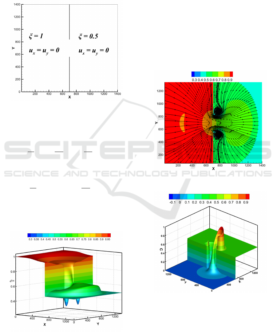
where
D
1
=
{
(x,y) : x ∈ [0,700], y ∈ [0,1400]
}
, (17)
D
2
=
{
(x,y) : x ∈ [700,1400], y ∈ [0,1400]
}
. (18)
Figure 5: Initial conditions for the 2D dam break problem.
The boundary conditions at x = 0 and x = 1400m are
assumed to be transmissive, or soft boundary condi-
tions:
∂h
∂n
= 0,
∂u
n
∂n
= 0,
∂u
τ
∂n
= 0, (19)
and all the other boundaries are considered as reflec-
tive:
∂h
∂n
= 0, u
n
= 0,
∂u
τ
∂n
= 0. (20)
At the moment of dam breaking, water is released
through the breach, forming a positive wave propa-
gating downstream and a negative wave spreading up-
stream.
Figure 6: 2D dam break – 3D plot for the water height at
t = 200s.
The solution is computed on a 500 × 500 grid,
which corresponds to ∆x = ∆y = 2.8 m. The same
grid was used in (Chertock and Kurganov, 2004; Delis
and Katsaounis, 2004). The results at time t = 200s,
with α = 0.5, β = 0.2 is shown in Figs. 6 – 9. As
one can observe, the scheme provides a very high res-
olution of the circular shock wave and the vortices
formed on the breach (Fig. 6 and 7).
As α decreases to 0.2, the amplitude of the vor-
tices increases, which corresponds to the picture pre-
sented in (Chertock and Kurganov, 2004; Delis and
Katsaounis, 2004). Similarly for concentration – fig.
8 and 9 - one can observe a clear arrangement of the
fronts and structures inside the vortices, as in (Cher-
tock and Kurganov, 2004).
Figure 7: 2D dam break – Contour lines of h and stream-
lines at the time t = 200s.
Figure 8: 2D dam break – 3D plot for the pollutant concen-
tration t = 200s.
The mentioned examples show that numerical algo-
rithm based on the RSWE system is comparable to
the developed methods of the high order of accuracy.
ONM-CozD 2019 - Special Session on Observations and Numerical Modeling of the Coastal Ocean Zone Dynamics
362
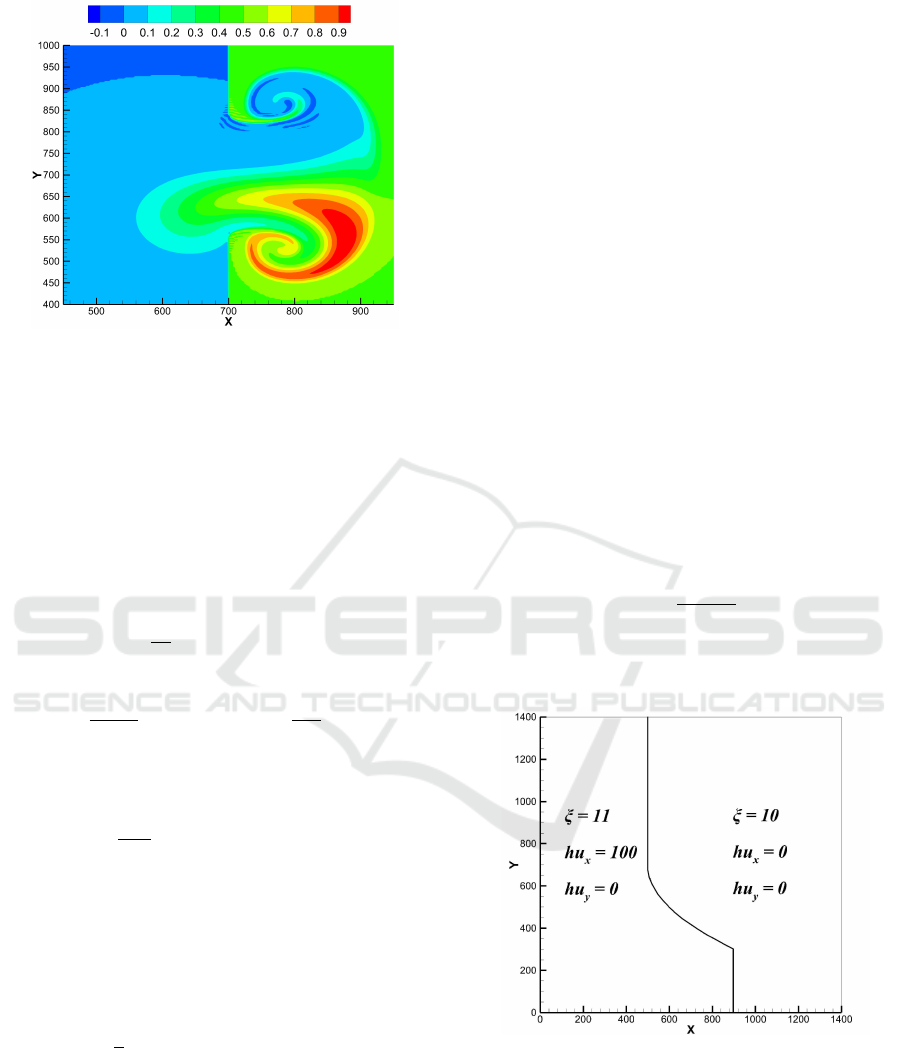
Figure 9: 2D dam break – top view for the pollutant con-
centration t = 200s.
5 TRANSPORT OF PASSIVE
POLLUTANT WITH SOURCE
TERM
The regularized system of shallow water equations in-
cluding a transport equation with source term has the
following form:
∂h
∂t
+ divj
m
= S, (21)
∂(hu)
∂t
+ div(j
m
⊗ u) + ∇
gh
2
2
= (22)
= −gh
∗
∇b + divΠ,
∂Ch
∂t
+ div(j
m
C) = T
s
S+ (23)
+div(Dh∇C + τu [(uh · ∇C) +CS − T
s
S]),
h
∗
= h − τ (div(hu) − S), (24)
j
m
= h (u − w), (25)
w =
τ
h
[div (hu ⊗ u) + gh∇(b + h)], (26)
Π = τu ⊗ [h (u · ∇)u + gh∇ (b + h) + Su]+ (27)
+τI [gh (div(hu) − S)].
Here we imply the same notations as in the
RSWE: h(x,t) and u(x,t) are the depth and veloc-
ity vector of the water respectively, b(x) describes the
topography of the bottom, g is the acceleration due
to the gravity, S(x,t) denotes the sources of water,
C(x,t) is an average pollutant concentration and T
s
is
a given value of a pollutant concentration at a sources
S. D is the diffusion coefficient.
Introducing a source term in shallow water equa-
tion system causes a number of computational prob-
lems in numerical realizations, (Audusse and Bris-
teau, 2003) and (Delis and Katsaounis, 2004). Partic-
ularly, for a system of equations with a source term,
it becomes necessary to preserve non-trivial equilib-
ria, which is very difficult for most known schemes.
One of the way to evaluate the influence of this fac-
tor on the solution, is the implementation of methods
of an energy estimations of the solution, developed in
(Zlotnik, 2012).
To demonstrate the performance of the RSWE
system with source term we take the test problem
from (Chertock and Kurganov, 2004), describing a
propagation of the pollutant from a non-stationary
source term in the region of the complex bottom
topology.
Consider the square domain: [0,1400]m ×
[0,1400]m with the initial water depth and velocity
distribution are shown in Fig. 10, where the shape of
the dam is given by:
Γ(y) =
min
h
500 +
(y−700)
2
400
,900
i
,
y ∈ [0, 700],
500, 700 6 y 6 1400.
(28)
Figure 10: Initial conditions for the 2D dam break problem
with non-zero source.
The bottom topography b(x,y) is given by three
elliptic-shape exponential humps:
b(x,y) = 4.5
h
e
−κ
1
(x−800)
2
−κ
2
(y−700)
2
+ (29)
e
−κ
2
(x−600)
2
−κ
1
(y−600)
2
+ e
−κ
2
(x−1000)
2
−κ
1
(y−700)
2
i
,
Numerical Simulation of Coastal Flows with Passive Pollutant by Regularized Hydrodynamic Equations in Shallow Water Approximation
363
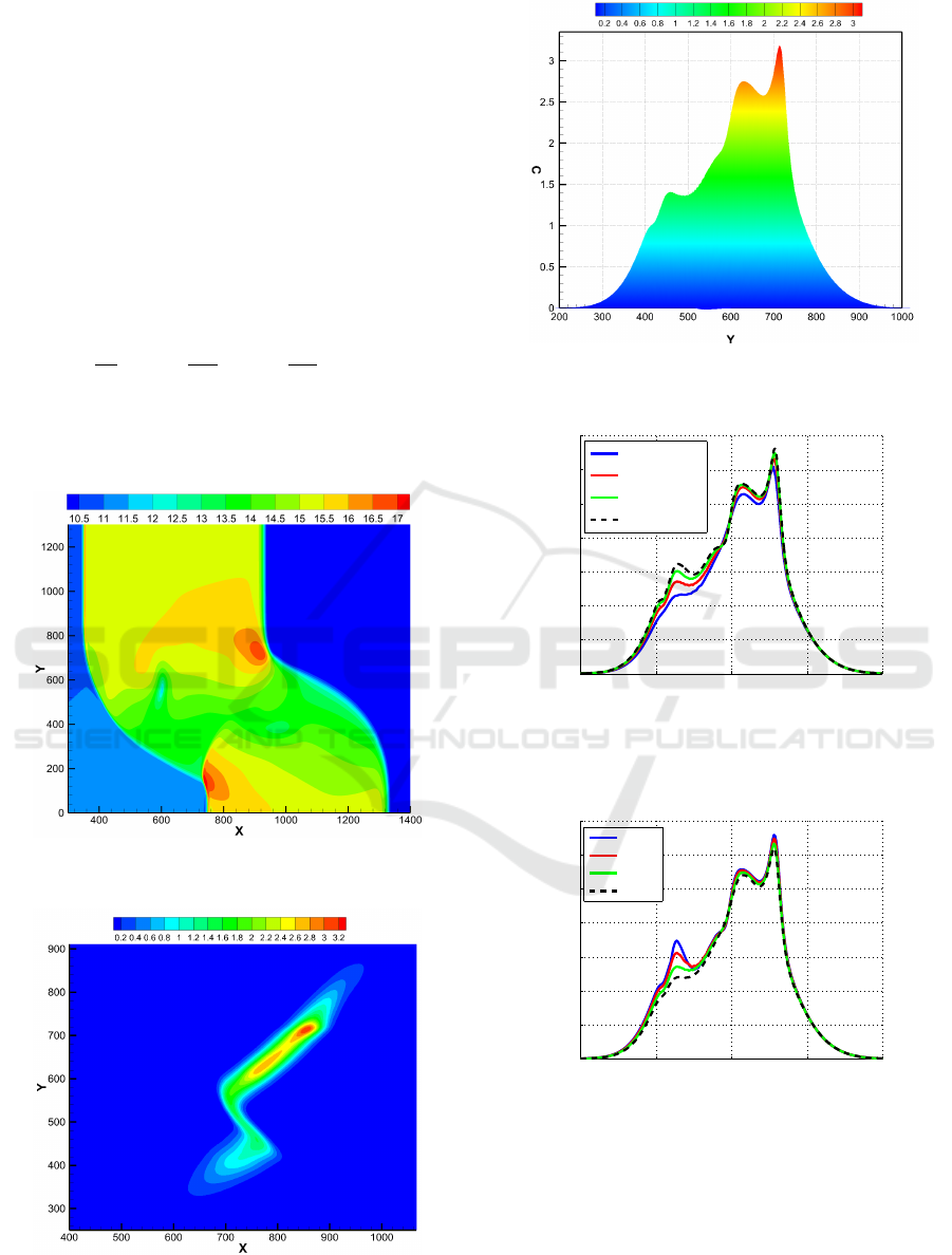
where κ
1
= 10
−4
, κ
2
= 10
−3
.
The initial concentration of pollutant is equal to
zero C(x,y,t = 0) = 0, but later, when on a source
of polluted water with the concentration of pollutant
T
s
= 25 is turned on:
S(x,y,t) = (30)
= 0.5e
−0.5(t−8)
2
−10
−5
(x+y−1300)
2
−5·10
−4
(x−y−100)
2
,
a pollutant begins to propagate in the domain.
The boundary conditions are considered as trans-
missive:
∂h
∂n
= 0,
∂u
n
∂n
= 0,
∂u
τ
∂n
= 0, (31)
The solution computed on a 500×500 grid, which
corresponds to ∆x = ∆y = 2.8 m and α = 0.5, β = 0.2
at time t = 30s is shown in Figs. 11–13.
Figure 11: 2D dam break with non-zero source – a contour
lines of ξ.
Figure 12: 2D dam break with non-zero source – a contour
lines of C.
Figure 13: 2D dam break with non-zero source – 2-D pro-
jections of C.
200 400 600 800 1000
0
0.5
1
1.5
2
2.5
3
3.5
Y,m
C
N
x
= N
y
= 200
N
x
= N
y
= 400
N
x
= N
y
= 800
N
x
= N
y
= 1600
Figure 14: 2D dam break with non-zero source – 2-D pro-
jections of C for α = 0.5, β = 0.2 and various partition of
the grid.
200 400 600 800 1000
0
0.5
1
1.5
2
2.5
3
3.5
Y, m
C
α = 0.2
α = 0.3
α = 0.5
α = 0.7
Figure 15: 2D dam break with non-zero source – 2-D pro-
jections of C for N
x
= N
y
= 400, β = 0.2 and various α.
In figure 11 one can observe that the collision of a
curved shock wave of the initial distribution with bot-
tom topography leads to rather complex wave struc-
tures.
Our results are compared with the semi-discrete
central-upwind finite-volume(FV) scheme and the hy-
ONM-CozD 2019 - Special Session on Observations and Numerical Modeling of the Coastal Ocean Zone Dynamics
364

brid finite volume particle method (FVP) for parti-
tioning on grid 500 ×500 in (Chertock and Kurganov,
2004).
The fig. 13 shows the results of calculations for the
concentration in a 2D-projection on the (C, y) axis.
The result obtained using the RSWE model was com-
pared with the FV and FVP methods from (Chertock
and Kurganov, 2004), and it was found that they are
placed approximately between them.
The dependence of the numerical solution on the
partition of the grid for the 2D-projection of C (β =
0.2, α = 0.5) is shown in fig. 14. Fig. 15 demonstrates
the 2D-projection of C (N
x
= N
y
= 400, β = 0.2) for
the various α.
6 CONCLUSIONS
The regularized shallow water algorithm with pro-
posed new method for pollutant transfer simulation
has the similar structure as the methods of numerical
solution of the subsonic and supersonic gas dynamics
flows, already successfully implemented in the Open-
FOAM platform (Kraposhin et al., 2018). The pro-
posed algorithms in a form of finite-volume method
can be included in the platform as a novel numeri-
cal solver for coastal flow simulations together with a
pollutant transfer.
ACKNOWLEDGEMENTS
This work is supported by the Russian Foundation for
Basic Research, project no. 190100262. The authors
thank to A.A. Zlotnik for constructive comments on
the regularized equations and for useful ideas on set-
ting initial conditions in pollutant transport problems.
REFERENCES
Audusse, E. and Bristeau, M.-O. (2003). Transport of pollu-
tant in shallow water a two time steps kinetic method.
ESAIM: M2AN, 37:389–416.
Bristeau, M.-O. and Perthame, B. (2001). Transport of pol-
lutant in shallow water using kinetic schemes. ESAIM:
Proc, 10:9–21.
Bulatov, O. V. and Elizarova, T. G. (2011). Regularized
shallow water equations and an eflcient method for
numerical simulation of shallow water flows. Com-
put. Math. Math. Phys., 51:160–173.
Chertock, A. and Kurganov, A. (2004). On a hybrid finite-
volume-particle method. ESAIM: M2AN, pages 1071–
1091.
Chetverushkin, B. N. (1999). Kinetically Consistent
Schemes in Gas Dynamic. Mosk. Gos. Univ., Moscow.
Delis, A. I. and Katsaounis, T. (2004). A generalized relax-
ation method for transport and diffusion of pollutant
models in shallow water. Computational Methods in
Applied Mathematics, 4:410–430.
Elizarova, T. G. (2009). Quasi-Gas Dynamic Equations.
Springer-Verlag, Berlin.
Elizarova, T. G. and Ivanov, A. V. (2018a). On a homoge-
neous algorithm for numerical modeling of a tsunami
wave. Memoirs of the Faculty of Physics, pages 1–6.
Elizarova, T. G. and Ivanov, A. V. (2018b). Regular-
ized equations for numerical simulation of flows in
the two-layer shallow water approximation. Comput.
Math. Math. Phys., 58(5):714–734.
Kraposhin, M. V., Smirnova, E. V., Elizarova, T. G., and
Istomina, M. A. (2018). Development of a new Open-
FOAM solver using regularized gas dynamic equa-
tions. Computers & Fluids, 166:163–175.
Saburin, D. S. and Elizarova, T. G. (2016). Numerical
modeling of seiche oscillations in the sea of azov us-
ing smoothed hydrodynamic equations. In Konovalov,
S. K., Korotaev, G. K., Ibraev, R. A., and Demishev,
S. G., editors, World Ocean: Models, Data and Oper-
ational Oceanology, page 49—50.
Saburin, D. S. and Elizarova, T. G. (2017). Application of
the regularized shallow water equations for numeri-
cal simulation of seiche level oscillations in the sea of
azov. Math. Models Comput. Simul, 9(4):423–436.
Saburin, D. S. and Elizarova, T. G. (2018). Modelling the
azov sea circulation and extreme surges in 2013-2014
using the regularized shallow water equations. rus-
sian journal of numerical analysis and mathematical
modelling. Russ. J. Numer. Anal. Math. Modelling,
33(3):173–185.
Sheretov, Y. V. (2009). Continuum Dynamics under
Spatiotemporal Averaging. NITs Regulyarnaya i
Khaoticheskaya Dinamika, Moscow.
Zlotnik, A. A. (2012). “spatial discretization of the one-
dimensional barotropic quasi-gasdynamic system of
equations and the energy balance equation. Mat.
Model, 24:51–64.
Numerical Simulation of Coastal Flows with Passive Pollutant by Regularized Hydrodynamic Equations in Shallow Water Approximation
365
