Gray-Box Models for Performance Assessment of Spark Applications

Marco Lattuada

1 a

, Eugenio Gianniti

1 b

, Marjan Hosseini

, Danilo Ardagna

1 c

Alexandre Maros

, Fabricio Murai

2 d

, Ana Paula Couto da Silva

and Jussara M. Almeida

Politecnico di Milano, Italy

Universidade Federal de Minas Gerais, Brazil

Keywords:

Spark, Big Data, Machine Learning.

Abstract:

Big data applications are among the most suitable applications to be executed on cluster resources because

of their high requirements of computational power and data storage. Correctly sizing the resources devoted

to their execution does not guarantee they will be executed as expected. Nevertheless, their execution can be

affected by perturbations which can change the expected execution time. Identifying when these types of issue

occurred by comparing their actual execution time with the expected one is mandatory to identify potentially

critical situations and to take the appropriate steps to prevent them. To fulﬁll this objective, accurate estimates

are necessary. In this paper, machine learning techniques coupled with a posteriori knowledge are exploited

to build performance estimation models. Experimental results show how the models built with the proposed

approach are able to outperform a reference state-of-the-art method (i.e., Ernest method), reducing in some

scenarios the error from the 221.09-167.07% to 13.15-30.58%.

1 INTRODUCTION

Many factors such as multi-tenancy, virtualization

and resource sharing can affect the performance of

federated cloud services and their resources. Mon-

itoring the status of the system during the applica-

tions runs to detect anomalies and perturbations can

be complex and can further degrade the overall per-

formance of the system. If the expected execution

time of the running applications was known a pri-

ori, the identiﬁcation of perturbed runs would be triv-

ial since it would just be a matter of comparing real

and expected execution time. In most of the scenar-

ios of practical interest, however, even the expected

execution time of running without perturbation can

be unavailable. For this reason, performance mod-

eling is used (Lazowska et al., 1984) to predict the

performance of a real application by abstracting its

behaviour.

Three main approaches have been proposed,

namely, white-box analytical models (AMs), black-

box machine learning (ML) models, and gray-box

https://orcid.org/0000-0003-0062-6049

https://orcid.org/0000-0002-5647-4024

https://orcid.org/0000-0003-4224-927X

https://orcid.org/0000-0003-4487-6381

ML models. AMs require the knowledge of the sys-

tem internals, which is not always available and typ-

ically relies on some simplifying assumptions at the

expense of losing accuracy (Lazowska et al., 1984).

On the other side, black-box models (Didona and Ro-

mano, 2015) based on ML try to learn from data and

make predictions without a detailed knowledge of the

system. Finally, gray-box models combine aspects

of the two approaches and consist of black-box mod-

els enriched with a set of features which better cap-

ture the behaviour of the applications under analysis.

ML models require a training phase in which they

use experimental data coming from different work-

loads and conﬁgurations. In order to obtain these ini-

tial data, it is necessary to run a set of experiments

which is costly and time consuming. Moreover, since

ML models are usually characterized by a wide set

of hyper-parameters, which inﬂuence their accuracy,

training should be done with hyper-parameter tuning

to achieve the best possible results. Therefore, the

training phase might take a long time. However, once

trained, the prediction of ML models is very fast and

usually very accurate. This is why ML models are re-

cently becoming popular in studying the performance

of large systems (Ataie et al., 2016).

In this paper, ﬁve classic ML models for regres-

sion are considered: `

-regularized Linear Regression

Lattuada, M., Gianniti, E., Hosseini, M., Ardagna, D., Maros, A., Murai, F., Couto da Silva, A. and Almeida, J.

Gray-Box Models for Performance Assessment of Spark Applications.

DOI: 10.5220/0007877806090618

In Proceedings of the 9th International Conference on Cloud Computing and Services Science (CLOSER 2019), pages 609-618

ISBN: 978-989-758-365-0

609

(LASSO), Neural Network, Decision Tree, Random

Forests, and Support Vector Regression. A ML li-

brary was also developed in order to automate the

training and evaluation of ML models and their hyper-

parameter tuning. We focus on assessing Spark appli-

cations performance, i.e., evaluate the execution time

measured for an application with respect to the ex-

pected one. Since the analysis is performed at the

end of applications execution, a posteriori knowledge

about them can be exploited. Examples of such type

of information are number of tasks, maximum and av-

erage task execution time, shufﬂe time and number of

bytes transmitted among the stages. To prove the gen-

erality of the proposed approach, a heterogeneous set

of applications including Spark SQL-based applica-

tions and ML benchmarks was considered.

The results of our experiments showed that there

is no single ML model which always performs well

or which always outperforms the others. According

to the initial application proﬁling data available in

the training set and the application data size, differ-

ent ML models provide signiﬁcantly different accu-

racy. Therefore, it is very important to have a library

to automate the training and hyper-parameter tuning

process. In this way, different scenarios can be effec-

tively investigated.

The rest of the paper is organized as follows.

Section 2 presents the related work while Section 3

presents the evaluated performance models. The ex-

perimental setup is introduced in Section 4 and the

obtained results are presented in Section 5. Finally,

the conclusions are drawn in Section 6.

2 RELATED WORK

The performance analysis and prediction of big data

applications running on the cloud can be tackled from

different perspectives. The most traditional ones rely

on analytical models (Nelson and Tantawi, 1988;

Mak and Lundstrom, 1990; Tripathi and Liang, 2000;

Ardagna et al., 2018) and simulation (Bertoli et al.,

2009; Wang and Khan, 2015). Yet, recent stud-

ies have employed supervised machine learning mod-

els for performance prediction (Venkataraman et al.,

2016; Mustafa et al., 2018; Pan et al., 2017; Alipour-

fard et al., 2017), which is the focus of this paper.

One such example is a regression model proposed by

the Spark creators (Venkataraman et al., 2016). The

model uses a reduced set of features, which are func-

tions of the data set size and of the number of cores.

The estimation of the model parameters was based on

non-negative least squares.

Mustafa et al. (Mustafa et al., 2018) proposed a

prediction platform for Spark SQL queries and ma-

chine learning applications, which, similarly to our

gray box models, also exploits features related to each

stage of the Spark application. This implies the exis-

tence of previous knowledge of the application pro-

ﬁle. However, some of these features (e.g., numbers

of nonShufﬂedRead, shufﬂedReadRecords and input-

Partitions

) are at a lower level compared to ours, and

thus require a ﬁner-grained analysis of the Spark log

to be computed. The authors reported prediction er-

rors of 10% for SQL queries and about 25% for ma-

chine learning jobs. As we will show, our approach

achieves better accuracy, and our experimental de-

sign considers more recent Spark workloads, includ-

ing deep learning use cases.

CherryPick (Alipourfard et al., 2017) is a sys-

tem that leverages Bayesian optimization to ﬁnd near-

optimal cloud conﬁgurations that minimize cloud us-

age costs for MapReduce and Spark applications. Un-

like other studies, the goal was not to accurately pre-

dict applications performance, but rather design a

model that is accurate enough to distinguish the best

conﬁguration from the rest. Similar ideas were also

exploited in the design of Hemingway (Pan et al.,

2017), which embeds the Ernest model and is special-

ized in the identiﬁcation of the optimal cluster conﬁg-

uration for Spark MLlib based applications.

In a related, but different direction, Nguyen et al.

(Nguyen et al., 2018) proposed a strategy to generate

training data to ﬁt a performance model. The model is

meant to be used for predicting which Spark settings

yield the smallest application execution time (i.e., ca-

pacity planning). In contrast, we here compare alter-

native ML models and feature sets in the task of pre-

dicting the performance of an application running on

a given conﬁguration.

3 ML MODELS FOR ASSESSING

THE PERFORMANCE OF

SPARK APPLICATIONS

This section presents the input features and the tech-

niques used to build the proposed regression models,

comparing them to the considered reference, model

Ernest (Venkataraman et al., 2016). The performance

models, which are built by means of Machine Learn-

ing (ML) techniques, consist of functions that relate

application characteristics, infrastructure settings, and

proﬁling information to the expected application exe-

cution time. The purpose of these models in the con-

https://spark.apache.org/docs/latest/rdd-programming-

guide.html

IWFCC 2019 - Special Session on Federation in Cloud and Container Infrastructures

610

sidered context is to assess the trustworthiness and the

absence of perturbations of the infrastructure w.r.t. the

execution performance. More precisely, the aim is to

determine whether an application run was affected by

performance degradation due to resource contention.

This task, which will be referred as Performance As-

sessment is of paramount importance in cloud man-

agement to verify that the resource allocation and iso-

lation did not lead, because of multiple applications

interference, to performance degradation. A second

possible task can be the capacity planning, i.e., to de-

termine the minimum amount of resources that must

be allocated so that the execution time is smaller than

a given limit. Differently from the ﬁrst task, the sec-

ond cannot rely on a posteriori knowledge and it will

not be considered in the rest of the paper.

The type of data available for ﬁtting the ML mod-

els depends on: (i) the application and (ii) the in-

frastructure settings. In this paper, three possible

classes of Spark applications are considered: SQL

based workloads, traditional machine learning algo-

rithms, and SparkDL (Deep Learning pipelines for

Spark).

3.1 Models Overview

Five classic ML models for regression are considered:

-regularized Linear Regression (LASSO), Neural

Network, Decision Tree, Random Forests, and Sup-

port Vector Regression. A short description of each

model is provided below.

• Linear regression (LR) assumes a linear relation-

ship between features and the outcome. This

model is typically ﬁt using variants of the least

squares method. The `

-regularized and `

regularized Linear Regression are respectively

known as LASSO, and Ridge Regression. It is

possible to force all coefﬁcients associated with

features to be positive by ﬁtting the data using the

non-negative least squares (NNLS) method. In

this paper, LASSO is considered which also helps

in reducing the number of features by frequently

setting weights to zero

. The NNLS method is

used by the reference method (Ernest (Venkatara-

man et al., 2016)).

• Decision tree (DT) is a model represented a

rooted, binary tree, composed of internal and leaf

nodes. Each internal node represents a test based

on the value of a feature. Leaf nodes aggregate

training data that satisfy the tests encoded by the

respective path. Algorithms used for constructing

such a tree include ID3 (Iterative Dichotomiser),

https://web.stanford.edu/∼hastie/ElemStatLearn/

C4.5 (a successor of ID3) and CART (Classiﬁca-

tion and Regression trees). Given a set of feature

values, a prediction is made by applying succes-

sive tests until a leaf is reached. The prediction

combines the outcome values associated with that

leaf.

• Random forest (RF) is an ensemble method,

which builds a collection of decision trees, to get

more accurate and less variable results. Each tree

is constructed by a random selection of features.

The predicted outcome is obtained by averaging

the predictions of all trees. Both ﬁtting and pre-

diction are efﬁcient (computationally simple) for

this method.

• Neural network (NN) is a model represented by

a set of connected input/output units (nodes) in

which each connection has a weight associated

with it. The network consists of an input layer,

one or more hidden layers and an output layer.

The inputs are given to the input layer, then

weighted and fed to the second layer which is a

hidden layer. The outputs of a hidden layer can

be given to another hidden layer or to the output

layer. Finally, the output layer gives the predic-

tion of the network for the given inputs. During

the network training, the difference between pre-

dicted value and true value (error) will be prop-

agated backward by apportioning them to each

node’s weights according to the amount of this er-

ror the node accounts for. This algorithm is called

backpropagation.

• Support vector regression (SVR) is a two step

model derived from support vector machines.

First step aims at addressing non-linearities: a

non-linear function is used to map original data

in a high dimensional feature space. In the second

step, hyper-planes are used to describe the linear

functions between points in the created space and

the metric to be estimated.

Linear regression was chosen because of its readabil-

ity and its usage in the Ernest models. Decision trees

and random forests while still partially interpretable,

are also able to describe non-linear relationships in

the data. Last, support vector regression and neural

networks are able to capture quite complex relation-

ships between applications characteristics and their

execution time.

3.2 Features Overview

Table 1 shows the features used by the considered

models. Two sets of features can be identiﬁed: fea-

tures which are available a priori and features which

Gray-Box Models for Performance Assessment of Spark Applications

611

Table 1: Features used in models for performance assessment.

Type of Knowledge Features

A Priori

- Ratio of data size to number of cores

- Log of number of cores

- Data size

- Number of cores

- Number of TensorFlow cores (SparkDL only)

A Posteriori

- number of tasks

- max/avg time over tasks

- max/avg shufﬂe time

- max/avg number of bytes transmitted between stages

- number of executor cores

- inverse of number of executor cores

A Posteriori (SparkDL)

- individual TensorFlow calls execution time

- inverse of total number of cores

are only available a posteriori. The former set is

composed of features which are derived by the Ernest

model and exploit information which is available be-

fore running the applications (more precisely, the

number of cores and the input data size) . The latter

set is composed of features which are associated with

the Spark DAG (directed acyclic graph), which repre-

sents the sequence of stages executed by Spark when

running an application

. This type of information can

be easily extracted from applications logs after their

completion. In general, since the DAG is speciﬁc to

each application run, the relationship between these

metrics and running time only holds for the same

DAG. To be able to achieve this, a ﬁxed DAG struc-

ture was needed, at least across different number of

cores. In particular, for each stage, the extracted in-

formation is: the number of tasks, the maximum and

average execution time of the tasks, the maximum and

the average shufﬂe time, the maximum and average

number of bytes transmitted among the stages. For

SparkDL, not only the cores assigned to Spark execu-

tors, but also the TensorFlow execution time and the

inverse of total number of cores available in the clus-

ter are included as features.

It is worth noting that full information (i.e., in-

cluding a posteriori knowledge) can be used since

built models are used to assess the performance of the

applications and not to predict it.

4 EXPERIMENTAL SETTINGS

This section presents and details the experimental

setup adopted in all the experiments performed to col-

lect the results presented in this paper. This section

ﬁrst describe the applications used as workloads in

our experiments (Section 4.1) and the considered tar-

https://data-ﬂair.training/blogs/dag-in-apache-spark/

get platforms on which applications were run (Sec-

tion 4.2). How the data were split into training and

test sets is described in Section 4.3, while the model

parametrization is presented in Section 4.4. Finally

the metrics adopted to evaluate the models are de-

scribed in Section 4.5.

4.1 Applications Workloads

To verify the generality of the proposed approach,

three different types of applications are considered,

which are representatives of different types of work-

loads:

• Query26, an interactive query from the TPC-DS

industry benchmark

representative of SQL-like

workload, which includes a small number of tasks

and stages (i.e., 10). It was run for various input

data set sizes: 250 GB, 750 GB, and 1000 GB.

• K-means, a ML benchmark from Sparkbench

K-means is the core of many ML applications

(clustering is an unsupervised learning technique,

which, however, is used very frequently to per-

form preliminary data set analyses even if in

the following classiﬁcation techniques are consid-

ered). It was run for Spark dataframes with 100

features, with values uniformly distributed in the

[0,1] range and the number of rows varying in 5,

10, 15 and 20 million. The DAG was the same

across all runs and for all the data sizes, contain-

ing 15 stages.

• Image classiﬁcation, a benchmark for image pro-

cessing internally developed and based on the

SparkDL library

. The developed application is

based on the novel deep learning pipelines which

http://www.tpc.org/tpcds

https://codait.github.io/spark-bench

https://databricks.github.io/spark-deep-learning/site/

index.html

IWFCC 2019 - Special Session on Federation in Cloud and Container Infrastructures

612

makes possible to develop high-level deep learn-

ing applications on Spark. In particular, this

framework supports transfer learning, one of the

most popular approaches used in the deep learn-

ing when the data set for training is small (Csurka,

2017), which enables to use pre-trained models on

different tasks. In particular, the application we

developed is a binary image classiﬁcation using

InceptionV3 as featurizer and linear SVM as clas-

siﬁer. The number of images in the input varied in

1000, 1500 and 2500 while the number of stages

is 8. As anticipated in Section 3.2, this bench-

mark is characterized by additional features and,

hence, is the most complex of the three consid-

ered workloads. SparkDL heavily relies on Ten-

sorFlow which affects the application completion

times. When SparkDL runs, the number of cores

allocated to Spark workers can be limited, but

spark-submit parameters cannot control the num-

ber of cores for TensorFlow, which uses all the

cores available in the cluster. For this reason,

also the TensorFlow number of cores (which cor-

responds to the number of cores available in the

cluster) and its inverse are included in the set of

used features.

4.2 Hosting Platforms

Applications were run on two platforms, Microsoft

Azure and a private IBM Power8 cluster, which are

representatives of different computing environments.

As a public cloud, Microsoft Azure is potentially af-

fected by resource contention. Thus, application ex-

ecutions might experience more variability. In con-

trast, IBM Power8 was fully dedicated to run the con-

sidered benchmarks without any other concurrent ac-

tivity (thus with no resource contention).

Query 26 and SparkDL were executed on Mi-

crosoft Azure using the HDInsight service with work-

ers based on 6 D13v2 virtual machines (VMs), each

with 8 CPU cores and 56 GB of memory running

Spark 2.2.0 on Linux. SparkDL application requires,

in addition, that TensorFlow and Keras are available

on the Spark cluster: versions 1.4.0 and 2.1.5 were

used, respectively. The executors memory was set to

10 GB. K-means was run on a Power8 deployment

that includes Hortonworks distribution 2.6, same as

Microsoft Azure, with 4 VMs, each with 12 cores and

58 GB of RAM, for a total of 48 CPU cores available

for Spark workers, plus a master node with 4 cores

and 48 GB of RAM. The executors memory, in this

case, was set to 4GB.

For Query 26 and K-means, experiments were run

varying the number of Spark cores between 6 and

44 cores (step of 2), repeating the execution with

the same conﬁguration 6 times. For SparkDL, the

number of cores was varied between 2 and 48 (step

of 2), repeating each experiment with the same con-

ﬁguration (i.e., the number of images and cores) 5

times. By considering different workloads, hosting

platforms and setup conﬁgurations, we build a rich

set of scenarios to test our prediction models.

4.3 Train and Test Sets Settings

Table 2: Workload data sizes in different scenarios.

Workload

Core Interpolation Data Extrapolation

Training Test Training Test

Query 26 [GB] 750 750 250, 750 1000

K-means [Rows] 15 15 5, 10, 15 20

SparkDL [Images] 1500 1500 1000, 1500 2000

To evaluate the ML models accuracy and analyze their

interpolation and extrapolation capabilities, the data

are split into training and test sets according to the

data size and by considering different cores conﬁgu-

ration. For each workload, in particular, two different

types of scenarios are considered, which are summa-

rized in Table 2

• core interpolation scenarios: only runs with the

same dataset size are considered (reported in Ta-

ble 2). Figure 1 shows the various scenarios (y-

axis) built for each workload based on different

splits of the data into training and test sets: in each

row (case number), blue boxes represent conﬁgu-

rations for which the data were used as part of the

training set (and cross-validation) and red crosses

indicate conﬁgurations used as part of the test

set

• data size extrapolation scenarios: the runs with

the largest dataset size (spanning across all avail-

able cores conﬁgurations) are put in the test set

while the runs with the other dataset sizes in

the training data, as shown in the two rightmost

columns of Table 2.

In the ﬁrst class of scenarios, the cases were de-

signed such that larger case numbers are associated

with harder predictions, as there training data include

samples from a smaller range of experiments w.r.t. the

number of cores. For example, for both Query 26 and

K-means, scenario C1 is built by alternating conﬁgu-

rations in the sequence of the number of cores (x-axis)

as training and test data. For Query 26, data from ex-

periments with the number of cores equal to 6, 10,

. . . , 40 and 44 are put in the training data (blue boxes)

The experiments with Query 26 on 20 cores were re-

moved because of anomalies (see Figure 1a).

Gray-Box Models for Performance Assessment of Spark Applications

613

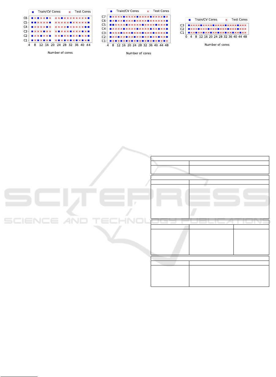
(a) Query 26 (b) K-means (c) SparkDL

Figure 1: Core interpolation scenario: train-test split in each case for Query 26, K-means and SparkDL.

while the remaining samples are included in the test

set (red cross). The gap between the number of cores

of consecutive conﬁgurations included in the training

data is gradually incremented. The gap in cases 4,

5, 6, and 7 was varied to assess its impact on model

accuracy. Since there is a large difference in the appli-

cation completion time in the runs where the number

of cores is small, the data for the smallest number of

cores were always included in the training set. For

SparkDL, the process was the same but limiting the

number of cases to three.

Even in the second class of scenarios, the train-

ing sets are further reduced by removing runs with

some conﬁgurations of number of cores according to

the same schema presented for core interpolation. By

doing so, in these experiments the core interpolation

and the data size extrapolation capabilities are evalu-

ated at the same time. In other words, the data size

extrapolation differ from the core interpolation sce-

narios because: (i) the dataset sizes in training and

test sets are no longer the same, (ii) the test set also

includes observations where the number of cores is

the same as in some observations of the training set

(but again with different dataset sizes).

4.4 Hyper-parameter Tuning

Each of the model described in Section 3.1 is char-

acterized by a set of hyper-parameters which can be

tuned to improve the accuracy of the models. Cor-

rectly sizing the design space on them is a critical

task, since a too narrow solution space can exclude

good solutions, while on the contrary a too wide solu-

tions space can lengthen too much the model selection

process. The hyper-parameters and the values which

were considered in this work are listed in Table 3. An

inhouse Python library was developed on the top of

PyTorch 0.4.0

(for neural network training) and of

scikit-learn 0.19.1

(for all the other techniques) to

explore their different values. For every algorithm,

the Mean Squared Error (MSE) integrated with hold-

https://pytorch.org

https://scikit-learn.org

out cross-validation was used to select the values that

led to the best model.

To further prevent over-ﬁtting, a regularization

term is added to LR (Linear Regression) and NN

(Neural Network). For LR, LASSO was chosen pro-

viding `

-norm. The use of intercept and the penalty

constant α are the set of available hyper-parameters

and are shown in Table 3 For the NN algorithm, the

Table 3: Hyper-parameters for ML techniques.

Linear Regression

Hyper-Parameter Values

Penalty α 0.001, 0.01, 0.05, 0.1, 0.5, 1.0, 5.0, 10.0

Fit intercept True, False

Neural Network

Hyper-Parameter Values

# Layers n 1, 2, 3

# Perceptrons/Layer all combinations in [3,4,5]

Activation Functions sigmoid, ReLU, tanh

Penalty 0.0001, 0.001, 0.01, 0.05, 0.1

Learning Rate 0.001, 0.01, 0.1

0.7, 0.8, 0.9

# Minibatches 1

Optimizer Adam, SGD

Decision Tree & Random Forest

Hyper-Parameter Decision Tree Random Forest

Max Depth 3, 5, 10, No Limit 3, 10, 20, No Limit

Max Features auto, sqrt, log auto, sqrt, log

Min samples to split 2.0 2.0

Min samples per leaf 1%, 5%, 10%, 20%, 30% 1, 2, 4

Criterion MSE, fMSE, MAE MSE, MAE

# Trees NA 5, 10, 50, 100

SVR

Hyper-Parameter Values

C 0.001, 0.01, 0.1, 1, 10, 50, 75

ε 0.05, 0.1, 0.2, 0.3, 0.5

γ 1e-7, 1e-4, 0.001, 0.01, 0.1, 1

Kernel linear, rbf, polynomial, sigmoid

Degree 2, 3, 5, 7

penalty Frobenius norm (Golub and Van Loan,

1996) was used. Also rectiﬁed linear unit function

ReLU was selected in general as the best activation

function. In all cases, the training data size was not

large; therefore, we set the number of minibatches

to 1 in order to consume the whole input at once.

The main hyper-parameter considered to evaluate the

performance was the optimizer. Adam and Stochastic

Gradient Descent (SGD) were evaluated as possible

candidates.

The former was selected as our experiments

showed that it converges much faster than the latter.

The number of epochs was set to 10,000. DT and RF

share many hyper-parameters and their values, there-

IWFCC 2019 - Special Session on Federation in Cloud and Container Infrastructures

614

fore, are grouped in Table 3. Max Depth is the max-

imum depth of the tree which is speciﬁed to avoid

over-ﬁtting. Max Features is used to select the num-

ber of available features to consider when searching

for the best split. A value of auto implies a maxi-

mum number of features equal to the total number of

features. Values of sqrt and log imply a maximum

equal to the square root and the base-2 logarithm of

the number of features, respectively. Minimum Sam-

ples to Split/per Leaf is used for setting, respectively,

the minimum number of samples required to split a

node and the minimum percentage/number of sam-

ples required to be a leaf. Criterion is the function

used to measure the quality of a split: MSE stands for

mean square error (minimizes `

loss), fMSE stands

for mean squared error with Friedman’s improvement

score for potential splits and, last, MAE stands for

mean absolute error (minimizes `

loss). Parameter

number of trees, the number of trees in the forest, only

applies to RF. A range of values is explored to analyze

diminishing return effects on the error. Finally, con-

cerning the SVR hyper-parameters, the degree is used

only with the polynomial kernel while the gamma pa-

rameter is valid only for polynomial, rbf and sigmoid

kernel. In the case of this regression technique, differ-

ent types of kernels are tried to observe which would

capture better the behavior of the application time ac-

cording to the number of cores.

4.5 Performance Metrics

To be able to compare the performance results of

different methods, the mean absolute percent error

(MAPE) of the response time assessment was used,

as it is more widely used in the performance liter-

ature (Lazowska et al., 1984) than MSE (used for

hyper-parameter tuning). Moreover, the results across

different experiments can be easily integrated even

if they have very different execution times. Indeed,

MAPE measures the relative error (in absolute terms)

of the prediction with respect to the true response

times, i.e.,

MAPE =

100%

∑

k=1



− ˆy



(1)

where

• N is the number of data points.

• y

is the response time measured on the opera-

tional system.

• ˆy

is the predicted response time from the learnt

model.

For each setup, 10 runs were executed for the LR,

DT and RF algorithms, and the average MAPE across

all 10 runs was computed and reported. For NN,

which has much longer training times, we performed

a single run (i.e., random train-test split).

5 EXPERIMENTAL RESULTS

In this section, the prediction results for each work-

load on each sets of scenarios (i.e., core interpolation

and data extrapolation) are presented. For each set,

this section reports the results in terms of MAPE for

each case described in Section 4.3 for each of the ML

technique described in Section 3.1 (LR, NN, DT, RF,

and SVR) comparing them with the reference model

(Ernest).

5.1 Query 26 Results

Table 4 and Table 5 show the MAPE results for core

interpolation and data extrapolation scenarios, respec-

tively, for Query 26. It is worth noting that in both

the sets of scenarios, Ernest method is quite accurate

(worst error is 8.02%) and outperforms gray box mod-

els since the features it exploits are better able to cap-

ture the characteristics of the application in terms of

performance. Moreover, there is no signiﬁcant differ-

ences in its accuracy across different cases, showing

that even with few observations it is possible to obtain

good ﬁts.

Analyzing the results of the gray-box models,

there is no ML technique which always outperforms

the other, but LR and NN are the best choices depend-

ing on the particular scenario.

Table 4: MAPE (%) of execution time estimates on Power8

for Query 26 in core interpolation scenario (ﬁxed data size

of 750 GB for all data sets).

Ernest

Gray Box

DT LR NN RF SVR

C1 1.50 9.64 4.46 7.10 6.71 7.35

C2 1.64 9.92 8.82 5.57 12.32 20.53

C3 1.71 16.12 6.23 4.24 15.31 10.25

C4 1.66 27.05 10.62 6.09 14.37 16.92

C5 1.59 25.54 42.08 6.23 44.60 39.74

C6 1.70 11.39 35.80 6.75 41.44 68.95

Even if they are not able to achieve the same accuracy

of the Ernest method, the worst result (32.29% on C4

of data extrapolation scenario) still allows to assess

the performance of the run application

5.2 K-means Results

Table 6 and Table 7 present the result obtained by

Ernest and by the ML techniques on K-means. Dif-

Gray-Box Models for Performance Assessment of Spark Applications

615

Table 5: MAPE (%) of execution time estimates on Power8

for Query 26 in data extrapolation scenario (250 GB,

750GB for training and 1000GB for testing).

Ernest

Gray Box

DT LR NN RF SVR

C1 7.49 37.13 32.91 10.23 44.16 38.08

C2 7.44 35.01 27.26 36.07 40.66 32.30

C3 7.31 32.39 36.36 20.18 47.46 38.74

C4 7.26 32.75 32.29 48.80 46.29 32.31

C5 7.59 41.93 12.41 21.90 31.50 18.11

C6 8.02 38.45 24.05 19.91 32.22 29.22

Table 6: MAPE (%) of execution time estimates on Power8

for K-means in core interpolation scenario (15M points for

training and 15M points for test).

Ernest

Gray Box

DT LR NN RF SVR

C1 126.69 17.27 74.04 11.99 105.31 28.09

C2 148.10 21.41 83.33 10.27 112.77 29.13

C3 161.35 46.46 122.07 47.30 67.58 36.14

C4 176.52 49.66 143.33 47.60 81.70 24.47

C5 187.00 31.20 273.19 29.88 99.74 84.00

C6 159.88 21.90 166.57 26.66 59.40 66.75

C7 178.08 31.59 159.44 47.65 102.96 38.74

Table 7: MAPE (%) of execution time estimates on Power8

for K-means in data extrapolation scenario (5M, 10M, and

15M points for training and 20M points for test).

Ernest

Gray Box

DT LR NN RF SVR

C1 167.07 26.47 20.24 59.50 26.07 16.04

C2 183.09 26.31 13.15 91.60 29.19 18.63

C3 200.83 37.28 31.86 131.54 33.47 30.58

C4 204.42 69.61 24.24 453.67 32.08 18.67

C5 221.09 26.89 26.86 16.01 39.72 25.29

C6 206.59 21.19 37.72 37.39 29.61 34.16

C7 208.37 29.44 43.14 145.81 30.21 24.06

ferently from the previous workload, the reference

model here is not able to correctly describe the ex-

pected performance of the considered application. In

the best case, the estimation error is 126.69% while

in the worst case it reaches up to 221.09%. On the

contrary, the errors of the best considered ML tech-

nique in each scenario are signiﬁcantly smaller. In

the worst case, C3 of core interpolation, the error of

the best technique (i.e., SVR) is 36.14% Even for this

workload, there is no ML technique which always

performs better than all the other in all the consid-

ered scenario. Indeed, all the techniques but RF are

the best choice in at least one combination of case-

scenario.

5.3 SparkDL Results

Finally, results for SparkDL are shown in Table 8 and

Table 9 for the core interpolation and data extrapola-

tion scenarios. Even if the predictions by the Ernest

method for this workload are better than for the pre-

vious, it still outperformed by other ML techniques.

In the core interpolation scenario the difference is not

so relevant since the error of the Ernest prediction is

in the range 5.71-10.48% while the error of the best

ML technique is in the range 3.70-4.66%. As for pre-

vious workloads, there is not an absolute best tech-

nique: NN, SVR, LR get the best results in each of

the three cases.

On the contrary, the data extrapolation for

SparkDL results to be a harder scenario to be ad-

dressed by the Ernest method with MAPE in the range

36.81-43.49%. Proposed models produce a signiﬁ-

cantly smaller error (range is 9.90-10.04%). Even in

this last scenario there is not a unique winner: LR is

the best technique for C1 and C2 while the best C3

model is built by NN.

Table 8: MAPE (%) of execution time estimates on Mi-

crosoft Azure for SparkDL in core interpolation scenario

(1500 images for training and 1500 images for testing).

Ernest

Gray Box

DT LR NN RF SVR

C1 10.48 5.16 5.60 3.84 5.87 4.12

C2 6.30 5.67 9.47 11.32 5.56 4.66

C3 5.71 6.40 3.70 5.07 8.29 4.96

Table 9: MAPE (%) of execution time estimates on Mi-

crosoft Azure for SparkDL in data extrapolation scenario

(1000 and 1500 images for training and 2500 images for

testing).

Ernest

Gray Box

DT LR NN RF SVR

C1 43.49 33.10 10.73 25.04 36.72 27.82

C2 37.39 34.94 10.04 17.64 35.47 32.13

C3 36.81 32.19 14.76 9.90 35.75 32.97

5.4 Discussion

The previous sections presented the results of the ref-

erence model and of the ML models for each ana-

lyzed workload and scenario. The Ernest models per-

form best (MAPE smaller than 8.02%) in the simplest

considered scenario (i.e., Query 26 both in core in-

terpolation and data extrapolation). In the SparkDL

core interpolation scenario, Ernest models still per-

form well despite not being the best models. In con-

trast, in the other scenarios, the large MAPE values

(up to 187%) make the models unsuitable for produc-

IWFCC 2019 - Special Session on Federation in Cloud and Container Infrastructures

616

tion environments, thus justifying the necessity of in-

troducing new techniques to be effectively exploited.

From the results previously presented, it can be

noticed that there is not a unique ML technique which

outperforms all the others in every situation. More-

over, even by limiting to a single type of scenar-

ios there is not a single winner. On the contrary, a

slight change in the composition of the training set

and of the test set (i.e., considering different cases)

may change which is the technique which performs

best. For example, in the data extrapolation scenario

for K-means the best technique is SVR for C1, C3,

C4, and C7, LR for C2, NN for C5 and DT for C6.

The comparison between the best gray box models

and the reference Ernest model leads to two different

situations. In scenarios where applications are char-

acterized by regularity (i.e., Query 26 and SparkDL

with ﬁxed data size), Ernest yields very good results

with MAPE values smaller than 11%, whereas the

best gray box model generally achieves worse perfor-

mance (MAPE of best models is in the range 3.84-

42.29%). Yet, in the remaining scenarios, which are

characterized by a larger variability in the application

execution times, the best gray box model outperforms

the Ernest model by a large margin. The MAPE range

of the latter is 36.81-187.0% while the largest error of

the best gray box model is only 31.59% (C of core in-

terpolation with K-means). However, recall that gray

box models use DAG-related features which are not

available for the test instance at prediction time (a pri-

ori), but they can be used as they are only to assess the

performance of the analyzed applications.

6 CONCLUSIONS AND FUTURE

WORK

In this paper, the accuracy of alternative supervised

machine learning techniques to assess the perfor-

mance of Spark applications has been analysed. Our

aim is to train models able at identifying perturba-

tions which affect the execution time of production

applications. Experimental results on a rich set of dif-

ferent scenarios demonstrated that the proposed gray

black box models are able to achieve relevant accu-

racy in different scenarios with different workloads.

Moreover, in complex scenarios (i.e., data extrapola-

tion in complex applications) where the Ernest refer-

ence model fails (error up to 187%), the largest er-

ror of the best gray-box model is 31.59%. However,

results show how there is no ML technique which

always outperforms the others, hence different tech-

niques have to be evaluated in each scenario to choose

the best model. As future work, the study of the

performance of Spark applications running on GPU-

based clusters is foreseen. Moreover, the use of the

models to identify resource contention on production

systems will be also considered.

ACKNOWLEDGEMENTS

This work has been partially supported by the project

ATMOSPHERE (https://atmosphere-eubrazil.eu),

funded by the Brazilian Ministry of Science, Technol-

ogy and Innovation (Project 51119 - MCTI/RNP 4th

Coordinated Call) and by the European Commission

under the Cooperation Programme, Horizon 2020

(grant agreement no 777154).

REFERENCES

Alipourfard, O., Liu, H. H., Chen, J., Venkataraman, S., Yu,

M., and Zhang, M. (2017). Cherrypick: Adaptively

unearthing the best cloud conﬁgurations for big data

analytics. In NSDI 2017 Proc., pages 469–482.

Ardagna, D., Barbierato, E., Evangelinou, A., Gianniti,

E., Gribaudo, M., Pinto, T. B. M., Guimar

aes, A.,

Couto da Silva, A. P., and Almeida, J. M. (2018). Per-

formance prediction of cloud-based big data applica-

tions. In ICPE ’18, pages 192–199.

Ataie, E., Gianniti, E., Ardagna, D., and Movaghar,

A. (2016). A combined analytical modeling ma-

chine learning approach for performance prediction of

mapreduce jobs in cloud environment. In SYNASC

2016, Timisoara, Romania, September 24-27, 2016,

pages 431–439.

Bertoli, M., Casale, G., and Serazzi, G. (2009). JMT: per-

formance engineering tools for system modeling. SIG-

METRICS Performance Evaluation Review, 36(4):10–

15.

Csurka, G. (2017). Domain adaptation for visual applica-

tions: A comprehensive survey.

Didona, D. and Romano, P. (2015). Using analytical models

to bootstrap machine learning performance predictors.

In 21st IEEE International Conference on Parallel

and Distributed Systems, ICPADS 2015, Melbourne,

Australia, December 14-17, 2015, pages 405–413.

Golub, G. H. and Van Loan, C. F. (1996). Matrix Com-

putations. The Johns Hopkins University Press, third

edition.

Lazowska, E. D., Zahorjan, J., Graham, G. S., and Sev-

cik, K. C. (1984). Quantitative System Performance.

Prentice-Hall.

Mak, V. and Lundstrom, S. (1990). Predicting performance

of parallel computations. IEEE Trans. on Parallel &

Distributed Systems, 1(undeﬁned):257–270.

Mustafa, S., Elghandour, I., and Ismail, M. A. (2018). A

machine learning approach for predicting execution

time of spark jobs. Alexandria Engineering Journal,

57(4):3767 – 3778.

Gray-Box Models for Performance Assessment of Spark Applications

617

Nelson, R. D. and Tantawi, A. N. (1988). Approxi-

mate analysis of fork/join synchronization in parallel

queues. IEEE Trans. Computers, 37(6):739–743.

Nguyen, N., Khan, M. M. H., and Wang, K. (2018). To-

wards automatic tuning of apache spark conﬁguration.

In CLOUD, pages 417–425.

Pan, X., Venkataraman, S., Tai, Z., and Gonzalez, J. (2017).

Hemingway: Modeling distributed optimization algo-

rithms. CoRR, abs/1702.05865.

Tripathi, S. K. and Liang, D.-R. (2000). On performance

prediction of parallel computations with precedent

constraints. IEEE Trans. on Parallel & Distr. Systems,

11:491–508.

Venkataraman, S., Yang, Z., Franklin, M., Recht, B., and

Stoica, I. (2016). Ernest: Efﬁcient performance pre-

diction for large-scale advanced analytics. In 13th

USENIX Symposium on Networked Systems Design

and Implementation, pages 363–378.

Wang, K. and Khan, M. M. H. (2015). Performance predic-

tion for apache spark platform. In HPCC-CSS-ICESS

2015 Proc., pages 166–173.

IWFCC 2019 - Special Session on Federation in Cloud and Container Infrastructures

618