
Real Time Financial Risk Monitoring as a Data-intensive Application
Petra Ristau and Lukas Krain
JRC Capital Management & Research GmbH, Kurfürstendamm 186, 10707 Berlin, Germany
Keywords: Financial Risk Measures, Value-at-Risk, Expected Shortfall, Monte-Carlo Simulations.
Abstract: This paper will examine the possibility of real-time risk calculations within the financial services industry.
Due to regulatory standards, this paper will focus mainly on the calculations of value-at-risk (VaR) and
expected shortfall (ES). Their computation currently requires simplified theory in order to be done within
real-time. This demonstrates a real-world disadvantage to investment professionals since they need to
comply with regulatory requirements when doing real-time decisions without knowing the accurate risk
numbers at any one time. Within the CloudDBAppliance project, we designed an architecture that shall
make real-time risk monitoring possible using cloud computing and a fast analytical processing platform.
1 INTRODUCTION
The financial services industry is heavily dependent
on risk simulations and calculations. This is even
more true in todays world since financial markets
change their behavior quicker and more drastically.
Regulatory entities, such as the German BaFin,
require finacial service providers to submit risk
figures such as value-at-risk (VaR) and may require
the submition of expected shortfall (ES) in the near
future. Due to their high complexity, it is common
practice to compute these figures in overnight batch
processes. Therefore, in between, investment
professionals need to estimate the according risk
measures and complete the decision-making process
without a clear understanding of their current
posistions. This presents an issue since the trader
opens and closes positions due to his perceived risk-
return profile. However, he does not know the
effects of his trade on the entirety of the trading
portfolios and the effects will only be calculated
overnight. In a worst-case scenario, the trader opens
a position on day t, the risk department computes at
night that the risk is too large to be kept in the books
and requires the trader to liquidate at a loss the next
morning.
The complexity of the risk calculations arises
from a Mont-Carlo simulation. In order to complete
this simulation, numerous statistics about financial
products need to be estimated which adds to the
computational requirements.
Although financial service providers face
different types of risks, we will focus only on market
risk, that is, the risk of falling investment values.
The remainder of the paper is structured as follows:
The next chapter introduces into the risk evaluation
task and discusses its computational complexity,
section 3 deals with requirements analysis while
section 4 introduces the platform architecture and
section 5 presents conclusions.
2 EXPLANATION OF RISK
FIGURES
In this chapter, we will have a look at how to
interpret a given VaR or ES figure and list all data
that is needed to do the calculations.
2.1 Value-at-Risk and Expected
Shortfall
According to modern portfolio theory (Elton et al.,
2014) the cross-correlations between financial
product’s prices have a big effect on the entire
portfolio value. This is why investment professionals
try to diversify risk by including uncorrelated or
even negatively correlated instruments into their
portfolio. This however, does not give the portfolio
manager an idea of possible losses beyond
deviations from the expected return. This is what
VaR does. VaR is technically a percentile of the loss
660
Ristau, P. and Krain, L.
Real Time Financial Risk Monitoring as a Data-intensive Application.
DOI: 10.5220/0007905706600665
In Proceedings of the 9th International Conference on Cloud Computing and Services Science (CLOSER 2019), pages 660-665
ISBN: 978-989-758-365-0
Copyright
c
2019 by SCITEPRESS – Science and Technology Publications, Lda. All rights reserved

distribution (Krokhmal et al., 2001) of an asset and
as such, VaR is a function of the asset returns, a
time-interval and a confidence level. VaR is stated in
a way such as “The 10-day, 99% VaR is equal to
72%”. Such a statement would mean that the risk
manager is 99% confident that the portfolio will not
lose more that 72% of its value within the next 10
days. ES gives an estimation of the loss given that
the loss exceeds the VaR. Continuing the above
example, an ES of 98% would be interpreted as
“Given that the loss is greater than 72%, the
expected value for the loss is 98%”. The ES can also
be translated as “There is a 1% chance of an event
that yields an expected return of -98%”.
2.2 Required Data
In order to calculate the VaR, we need an
appropriate length of price history. The variance-
covariance matrix needs to be calculated and a few
parameters need to be chosen i.e. which simulation
technique (Monte-Carlo-Simulation or historical
simulation), the number of simulations and which
distribution defines the given data best (in the case
of the Monte-Carlo-Simulation). The last factor, the
underlying distribution, can be estimated using the
historical data as well.
2.3 Mathematical Derivation of Value
at Risk and Expected Shortfall
In this article we will not discuss the selection of the
most appropriate method and the problematic of the
normal distribution assumption and refer to (Jorion,
2006) and (Embrecht et al., 2005). We decided to
exclude the parametric approach and instead use a
quantile function/distributional approach. We have
to simulate return data and then deduct information
from the simulated distributions. While Engle,
Manganelli (Engle and Manganelli, 2001) state VaR
as the solution to
Pr
|
,
where
is the loss at time t,
is all the collected
information at the time prior to the calculation and
theta is the desired confidence level, Ziegel (2013)
describes VaR as the solution of
inf∈|
,
with
being the cumulative distribution function of
the return distribution.
Assuming that we managed to compute the VaR
number for a given return distribution, we can easily
compute the ES using a simple mean over all
simulated returns that breach the VaR figure.
Therefore, the ES is given by
∈
|
,
where
is used as described above.
As already discussed, there are two main
simulation methods for generating the returns, from
which the quantile functions can start. Because the
historical simulation takes the actual past price
history for scenario building, it is heavily dependent
on the assumption that the training data is
representative for the underlying asset’s overall
returns. In the crucial case of stress scenarios that
never happened before it will thus underestimate the
risk.
This problem is solved by the Monte-Carlo
simulation, which estimates the underlying
distribution and generates thousands of simulated
future scenario based on it. The quantile functions
then calculate the risk figures based on the
distribution of the future scenarios. The academic
literature tends to link the Student’s t-distribution to
capital market returns (Harris, 2017), so the risk
manager has been given a hint about which
distribution to use.
2.4 Calculation Efficiency
Next, we will look at the runtime of a VaR
calculation based on a Monte-Carlo simulation. We
will see where the trade-off between speed and
accuracy of the calculation arises.
The first factor to consider when talking about
the runtime of a VaR calculation is the size of the
training data. As discussed above we only need the
asset returns for the calculations. The length of the
training data and the number of assets within the
portfolio increase the size of the training data
linearly. Obviously, a portfolio with x assets and a
training data set of the most recent T asset returns
has data points. The training data can be
represented in a matrix
∶
,
,
where and 1, and
,
,
is the return of
asset x at time t.
The next factor to consider is the variance-
covariance matrix. If our portfolio includes x assets,
the variance-covariance matrix will be -
dimensional and therefore, it has
entries with the
single asset’s variance on the main diagonal and the
covariance of asset i and j in the i-th row and j-th
column. Obviously, the variance-covariance matrix
is symmetrical, since the covariance function is
Real Time Financial Risk Monitoring as a Data-intensive Application
661
symmetrical. With
entries in a symmetrical
matrix we need to calculate
/2 entries,
which grows quadratically with an additional asset
in the portfolio. Next, we look at the necessary
number of computations for the variance and
covariance. Using the regular formula for the two
statistics, we get
,
∶
,
∗
,
and
∶
,
,
where is the expectation operator and
,
are the
returns of two assets within the portfolio. The
expectation operator requires linear runtime over the
length of the training data. If the training data has
length T, then the variance requires 2
calculations. The covariance requires 4
calculation because two different variables are
observed. This leads to a computational effort of
1
∗
4
2
2
for the entire variance-covariance matrix using the
standard equations and a brute force approach for
calculating them.
The next step in calculating the VaR is
estimation of the underlying distribution.
Independently from the chosen distribution the
simulation of a vector
̃
which is the generated returns of the simulated
future of length n. If the returns in the training data
are daily returns then the simulated future of length
n would be appropriate for a n-day VaR. This
procedure needs to be repeated multiple times for a
simulation. The sum of each individual vector ̃ is
the overall return of the portfolio over the required
time-period. Any function of the ones shown above
can be used to calculate the required percentile of
the sums of the ̃.
This calculation requires a lot of computational
runtime, mainly due to the quadratic growth of the
variance-covariance matrix and the generation of the
multivariate distribution. Furthermore, the number
of simulated random vectors ̃ should be very high.
In fact, even though the size of the training data has
an optimum unequal to the maximum, the number of
simulated portfolio returns will always increase the
accuracy of the VaR figure. An increased number of
simulated return vectors however, increases the
computational requirements as well. Yet, the
computations of all ̃ is the same and in fact, need to
be independent from each other (that is, the
generation of one random return vector must not
depend on the generation of another random return
vector). Therefore, a parallel computation of the
random return vectors will decrease the runtime in a
very efficient manner because the calculations of the
random return vectors can the distributed to all
processors equally. Furthermore, there exist efficient
parallel algorithms to compute the variance and the
covariance much more efficiently.
3 REQUIREMENTS ANALYSIS
The real-time risk monitoring for investment
banking use case shall implement a risk assessment
application that does, on the one hand, comply with
regulatory requirements of the financial supervisory
authorities, and on the other hand, speeds up the risk
valuation. That is, it can be used intraday not only
for regularly or ad-hoc queries, but even for pre-
trade analysis of potentially new trades before the
traders actually give the order.
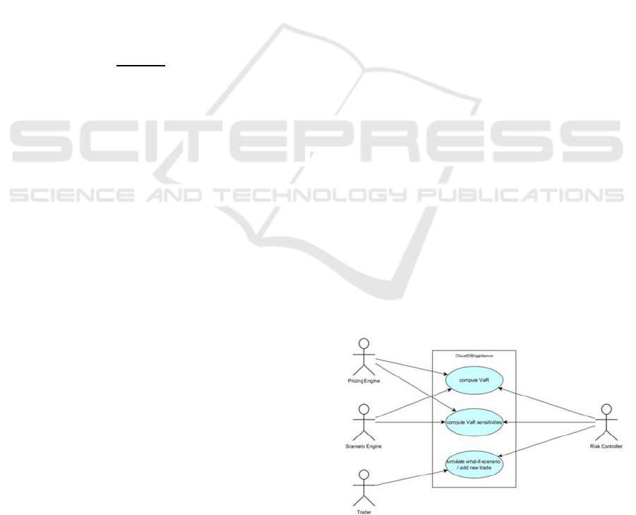
3.1 Use Case Analysis
Two types of human actors will interact with the risk
monitoring platform:
The Risk Controller will have access on all use
cases, i.e. the calculation of risk measures (VaR and
ES) as well as the corresponding sensitivities. The
pre-trade analysis may be triggered by the Risk
Controller as well as by the Trader who has just
detected an investment opportunity and would like
to evaluate the portfolio risk as if the new trade was
already carried out. This is what the ‘what-if’
analysis will compute.
Figure 1: Risk monitoring use case diagram.
The other two actors depicted in the above
diagram represent the pricing engine and the
ADITCA 2019 - Special Session on Appliances for Data-Intensive and Time Critical Applications
662

Figure 3: Activity diagram.
scenario engine that carry out the calculations as
described in section 2, but can be replaced by
instances using other calculation approaches.
While the scenario engine contains simulated
risk factors the pricing engine is a program that
makes real time price calculations based on real time
market data.
3.2 Input and Output Streams
The basis for every risk evaluation is the trade
history, consisting of string variables identifying the
currently open positions and past closed positions, in
combination with the history of market price data.
The result is a time series of numeric returns of the
portfolio that will serve as input for the pricing
engine that will generate a sufficient number of
pricing scenarios in order to put the risk valuation on
a profound basis. The resulting returns are deducted
from the price data input, which is a time series of
the most recent bid and ask prices. Due to the real-
time character of the data, each position within the
portfolio will generate new numeric data every tick,
i.e. every time a new price for the security is
available. The pricing engine will average all prices
within one second in order to generate an evenly
spaced data-stream. In case of no price change
within a one-second period, the most recent price
will be used. The input and output streams depicted
in figure 2 below consist of:
Open Positions: The basis for every risk evaluation
is the trade history, consisting of currently open
positions and past closed positions, in combination
with the history of market price data. All currently
open positions and their relative amount held form
the portfolio. The relative amount held is stored as
numeric data and will be called ‘weight of the
position’. The result is a time series of returns of the
portfolio that will serve as input for the pricing
engine that will generate a sufficient number of
pricing scenarios in order to put the risk valuation on
a profound basis. We estimate ‘sufficient’ to be no
less than 20.000 scenarios in regular financial
market times but much higher numbers during
stressed scenarios reaching 100.000 scenarios and
more. The estimate of 20.000 scenarios follows from
analyses of the stability of the risk calculation.
Potential New Trade: In order to provide also pre-
trade analysis, the trader may enter the position
he/she may intend to enter and may start a what-if
analysis that evaluates the changes of the risk
measure that would be caused by this additional
trade.
On the output side we receive the risk measures
VaR and ES for the current portfolio together with
their sensitivities to a range of parameters.
In case that a pre-trade analysis was triggered the
output will consist of the newly calculated risk
measures VaR and ES for the expanded portfolio
(what-if-scenario VaR).
Figure 2: Inputs and Outputs.
3.3 Activity Diagram
The sequence of operations is rather straightforward,
as can be seen from figure 3 above. From the login
of the risk controller or trader up to the calculation
of the VaR and ES risk measures the internal task
sequence depends on the availability of pricing
Real Time Financial Risk Monitoring as a Data-intensive Application
663
information. If pricing scenarios exist, the risk
measures VaR and ES can be calculated directly.
Otherwise, a sufficient number of price scenarios
has to be generated and fetched. Subsequently, the
related sensitivities are computed with respect to a
given set of parameters. If a new pre-trade analysis
is requested, the risk measure of the existing
portfolio has to be updated in the same way, before
the additional trade will be added and the new risk
measures are calculated incrementally.
4 PLATFORM ARCHITECTURE
In the real-time risk monitoring use case, we aim to
develop a solution capable of doing highly non-
linear financial risk computation on a large portfolio
of trades changing in real-time (new trades coming
in, what-if scenarios, etc.). The goal is to utilize in-
memory capabilities of the solution to avoid
expensive brute-force re-computations and make it
possible to both compute risks much faster but also
to allow marginal computations of risk for new
incoming transactions. The risk monitoring
application is designed to use fast analytical and
streaming processing capabilities of third-party
systems, i.e. the Big Data Analytics Engine, the
Operational DB and the Streaming Analytics Engine
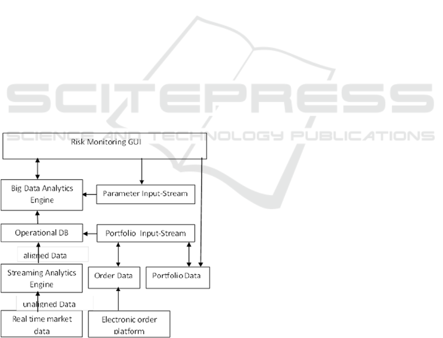
shown in figure 4 below.
Figure 4: Use case architecture and data flow.
The input data streams are located at the bottom
of the diagram. The real time market data is one
high frequency data stream of financial price data
for stocks, bonds, futures, currencies, etc. as offered
by numerous providers like Bloomberg, Reuters, or
Metastock. The task of the streaming analytics
engine is to filter only those assets that are contained
in the current portfolio and to align all incoming data
into streams with synchronous time stamps (e.g. on
1 second basis). This is a prerequisite for the
calculation of the variance-covariance matrix.
The aligned data is then stored in the
operational data base and immediately passed
through into the Big Data Analytics Engine. The
Analytics Engine can be configured via a GUI
where also the results are presented to the user.
Concerning the second type of input, the trade
history, we can distinguish between order data and
portfolio data. The order data consists of all trades
and is derived directly from the electronic order
platform. Each broker offers a dedicated order
platform where traders enter the new trades that are
then instantaneously forwarded to the account held
by the broker. The portfolio data is entered by the
risk manager directly from the GUI and contains
information about the asset allocation of the
portfolio.
The Portfolio Input-Steam is an API dedicated
to the storage of the order and portfolio data in the
data base.
Finally, the Parameter Input-Stream is fed
from the GUI and contains all parameters for the
scenario generation that usually remain fixed, but
might be subject to change in the case that the risk
controller needs to make adjustments.
5 CONCLUSION
The presented risk monitoring use case is a data-
intensive application in a critical infrastructure. It
does not require many different functionalities, but
focusses on a central aspect in the daily risk
management procedures of banks and financial
institutes.
The challenge of the application lies in the
computational complexity of the calculation of the
risk measures. This is where it will exploit the
capabilities of the underlying existing big data and
streaming analytics platforms. Using the projects’
platforms, it will be possible to calculate risk figures
in real-time and therefore prevent the trader from
entering into trades that yield a harmful risk
structure.
The chosen architecture design is kept modular
and will allow for the replacement of single
components, either on the side of data base or
ADITCA 2019 - Special Session on Appliances for Data-Intensive and Time Critical Applications
664

analytical platform, but also with respect to the data
sources like the real time market data feed or
electronic order platform by simply replacing the
interface. This will keep the design sustainable and
open for future extensions of requirements.
ACKNOWLEDGEMENTS
This project has received funding from the European
Union’s Horizon 2020 research and innovation
programme under grant agreement No. 732051. The
authors acknowledge consortium members support
in the described work and efforts in the
implementation of the platform components.
REFERENCES
Elton, E., Gruber, M., Brown, S., Goetzmann, W., 2014.
Modern Portfolio Theory and Investment Analysis.
John Wiley & Sons, 9
th
edition.
Embrechts, P., Frey, R., McNeil, A., 2005. Quantitative
risk management: Concepts, techniques and tools.
Princeton university press: Princeton, Vol. 3.
Harris, D.E., 2017. The Distribution of Returns. Journal of
Mathematical Finance, 7, 769-804.
Jorion, P. 2006. Value at risk: the new benchmark for
controlling market risk. Chicago: IRWIN, 3
rd
edition.
Krokhmal, P., Palmquist, J., Uryasev, S. 2002. Portfolio
Optimization with conditional Value-at-Risk Objective
and Constraints. Journal of risk 4, 43-68.
anganelli, S., Engle, R., 2001. Working paper. Value
risk models in finance. European Central Bank
Working Paper Series. Available at SSRN:
https://ssrn.com/abstract=356220.
Ziegel, J., 2013. Coherence and Elicitibility. Mathematical
Finance 26.4, 901-918.
Real Time Financial Risk Monitoring as a Data-intensive Application
665
