A Generic Control Framework for Mobile Robots Edge Following

Mathieu Deremetz

1 a

, Adrian Couvent

1 b

, Roland Lenain

1 c

, Benoit Thuilot

and Christophe Cariou

1 d

Universit

e Clermont Auvergne, Irstea, UR TSCF, Centre de Clermont-Ferrand,

9 avenue Blaise Pascal CS 20085, F-63178 Aubi

ere, France

Universit

e Clermont Auvergne, CNRS, SIGMA Clermont, Institut Pascal, F-63000 Clermont-Ferrand, France

christophe.cariou@irstea.fr

Keywords:

Wheeled Robots, Field and Agriculture Robots, Edge Tracking.

Abstract:

In this paper, the problem associated with accurate control for mobile robots following an edge is addressed

thanks to a backstepping control. In particular, the control of the angular speed (control input) is investigated

through the derivation of a new backstepping control by gathering derivatives regarding to time and to the

curvilinear abscissa in a single framework. This new reference then allows both time and distance convergence

of the robot states towards a trajectory computed with points given by a Lidar only. This permits to address

the control of different kinds of robots (skid-steering, car like, four-wheel-steering) in a common framework

and to consider independently the speed regulation, the lateral and the longitudinal controls. The control

proposed here allows an accurate and reactive path tracking even if the environment is complex and narrow.

The efﬁciency of the approach is investigated through full scale experiments in various conditions.

1 INTRODUCTION

Mobile robotics has raised as a promising solution to

help people in everyday life and has been the subject

of a lot of signiﬁcant advances. The progress achieved

on autonomous cars (Marmoiton and Slade, 2016) is

one of the best examples, since ﬁrst commercial so-

lutions are about to be marketed. Human transporta-

tion is not the sole application area which may beneﬁt

from autonomous mobile robots and numerous social

needs may be addressed thanks to this topic (Berger-

man et al., 2016). This is particularly the case in envi-

ronment and agriculture areas, where painful and dan-

gerous works have to be achieved. As a result, the use

of robots able to act autonomously to pull an imple-

ment or to carry out heavy loads may permit, among

others, the reduction of the hardness of work or the

limitation of the operator exposition to risks (Black-

more, 2016).

In this context, the autonomous motion task of-

ten consists in trajectory following, which has been

deeply studied in the literature (Samson et al., 2016).

https://orcid.org/0000-0002-1239-0320

https://orcid.org/0000-0002-3453-1358

https://orcid.org/0000-0003-0348-8673

https://orcid.org/0000-0002-7343-7452

In open area, this can be easily achieved using a GPS

sensors, offering permanently an absolute localization

for the robot navigation (Cariou et al., 2010). Never-

theless, this sensor appears to be expensive and not al-

ways applicable, especially in vineyard or orchard ap-

plications. The height of the vegetation in these con-

texts may indeed lead to a bad reception of satellite

signals. Moreover, since agricultural tasks have to be

done with respect to crops, the regulation of the robot

motion with respect to vegetation must be favoured.

As a result, alternative approaches have been pro-

posed, often based on artiﬁcial vision such as consid-

ered in (Cherubini and Chaumette, 2013), in (Tour-

rette et al., 2017), or in (Astrand and Baerveldt, 2005)

for agricultural applications, or based on a Lidar, such

as achieved in (Bayar et al., 2015). As soon as a lo-

cal positioning is available, different control laws can

then be applied (such as derived in (D’Andr

ea-Novel

et al., 1995), or (Lenain et al., 2017)). Nevertheless,

such approaches do not explicitly compute the an-

gular orientation and are therefor not suitable when

moving autonomously in narrow spaces, such as en-

countered for instance in vineyard, or when achiev-

ing harsh manoeuvres. Another approach introduced

in (Deremetz et al., 2017) allows to control the abso-

lute orientation of the robot with respect to the global

104

Deremetz, M., Couvent, A., Lenain, R., Thuilot, B. and Cariou, C.

A Generic Control Framework for Mobile Robots Edge Following.

DOI: 10.5220/0007915501040113

In Proceedings of the 16th International Conference on Informatics in Control, Automation and Robotics (ICINCO 2019), pages 104-113

ISBN: 978-989-758-380-3

frame, but this latter is not available in the considered

applications.

In this paper, an alternative approach of the tra-

jectory tracking to follow an edge is proposed. It

is based on a backstepping control, allowing to con-

sider independently longitudinal and lateral controls

and separate the position and the orientation servo-

ing of the robot. This permits to improve the control

of the robot orientation to improve manoeuvrability

and avoid the collision with the structure to be fol-

lowed. This control is generic and developed for sev-

eral kinds of robots: skid-steering, car-like mobile,

or four-wheel steering robots. In the latter case, the

backstepping approach is enhanced in order to regu-

late the actual orientation of the robot in order to opti-

mize the work of an on-boarded implement (which is

important for agricultural tasks, such as spraying) as

well as the manoeuvrability.

This paper is decomposed as follows. First, the

kinematic model of a mobile robot with respect to an

edge is recalled. Based on this generic modelling,

the proposed backstepping control approach is de-

tailed. Then additive features to improve manoeu-

vrability and safety are presented. Finally, the efﬁ-

ciency of the proposed control architecture is investi-

gated through full scale experiments in various condi-

tions, using several kinds of robots.

2 MODELLING

2.1 Assumptions and Notations

In this paper, the objective is to follow a structure,

using an edge detector, thanks to a mobile robot. For

that purpose, a control strategy based on the trajectory

tracking point of view may be considered, as classi-

cally investigated in (Samson et al., 2016). In this

point of view, a four-wheel-steering robot can be de-

scribed as a bicycle such as depicted in Fig 1. The

robot is reduced to two wheels, one for the front axle

with a steering angle denoted as δ

, and one for the

rear axle, with an angle denoted δ

The position of the robot is deﬁned with respect to

the detected structure Γ to be followed (considered as

a trajectory), with a lateral error y, also called track-

ing error, and a curvilinear abscissa s (i.e. the dis-

tance achieved along the trajectory). Let us denote by

θ, the difference between the orientation of the robot

and the direction of the tangent to Γ at the curvilin-

ear abscissa s. The curvature of the trajectory to be

followed at the curvilinear abscissa s is denoted by

c(s). With these notations the objective of the struc-

ture following strategy is to ensure the convergence

Figure 1: Modelling of the mobile robot w.r.t. the detected

structure Γ.

of the lateral deviation y to some desired set point y

at a desired speed v

. As it will be pointed out in the

following, even if a four-wheel-steering robot is pre-

sented in this section, the proposed control strategy is

also derived for a skid-steering robot or a car-like mo-

bile robot (with only an inactive rear steering δ

= 0).

The state vector associated to this framework may be

deﬁned as follows:

X =









. (1)

2.2 Motion Equations

Based on the notations introduced previously and ac-

cording to (Samson et al., 2016), one can obtain the

derivative of the state vector X with respect to time,

which constitutes the evolution model for the path

tracking problem.

X =







˙s =

v cos (

θ + δ

)

1 − y c(s)

˙y = v sin(

θ + δ

)

θ = u

−

c(s)v cos(

θ + δ

)

1 − y c(s)







. (2)

The variable u

denotes the yaw rate of the robot,

which is directly a control variable for a skid steering

robot. For a four-wheel-steering robot, this variable

depends on the values of the steering angles, which

are the actual control variables. The relation between

and these steering angles can be deﬁned by the fol-

lowing relationship:

= v cos(δ

)

tan(δ

) − tan(δ

)

, (3)

with L denoting the robot wheelbase. For a car-like

mobile robot, the model (2)-(3) still stands by impos-

ing a null rear steering angle (δ

= 0).

A Generic Control Framework for Mobile Robots Edge Following

105

In this paper, another objective is to follow a struc-

ture relying on the travelled distance of the robot (that

is to say independently from the robot’s speed). As

a result, the model (2) can be rewritten according to

derivatives w.r.t. the curvilinear abscissa s instead of

w.r.t. time. Let us deﬁne by X

, the derivatives

of the variable X w.r.t. s. From (2) it can be expressed

as:







= 1

= (1 − y c(s))tan(

θ + δ

)

= u

1 − y c(s)

v cos(

θ + δ

)

− c(s)







. (4)

The expression (4) exists for the last equation (yaw

motion) if the longitudinal velocity v is not null. This

assumption is not a limitation in the following since

the synthesis of the control avoids this singularity.

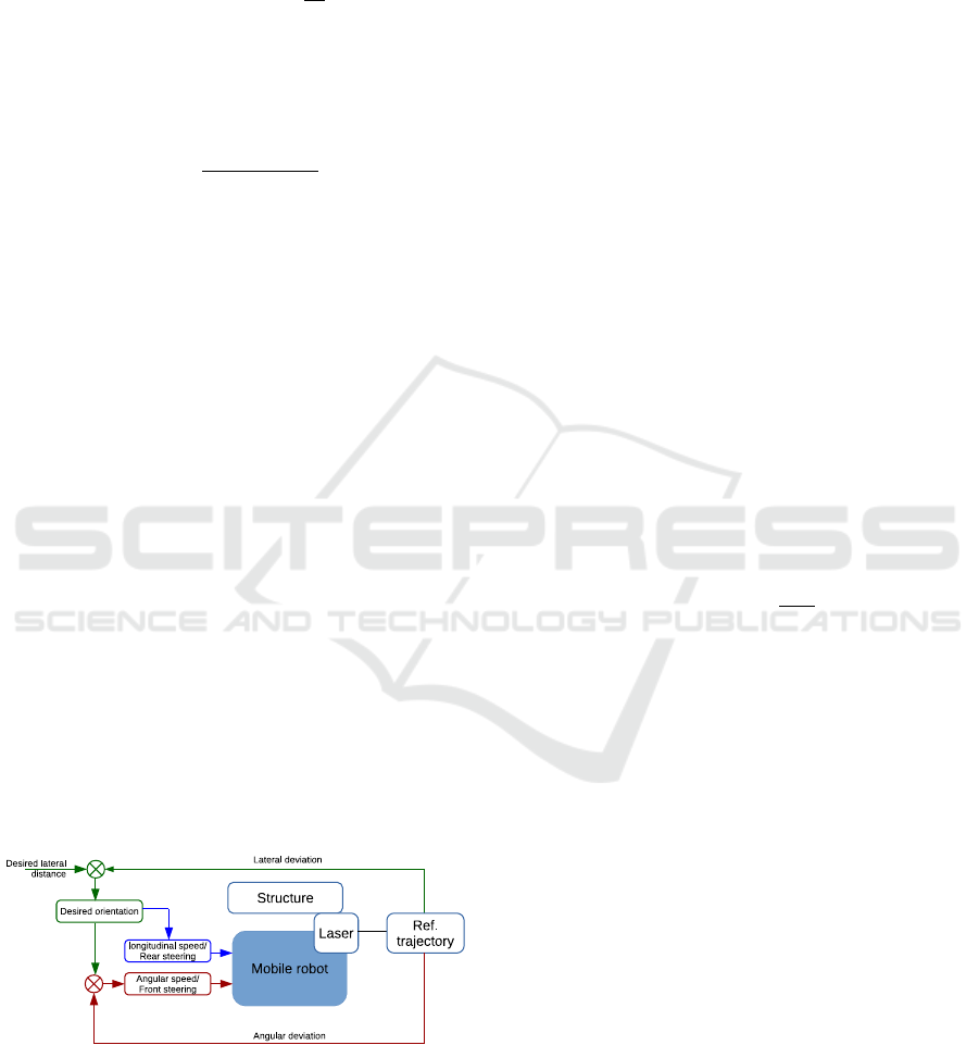
3 PROPOSED CONTROL

ARCHITECTURE

The control strategy proposed in this paper is based

on a backstepping approach, which is summarized in

Fig. 2. Using this principle, this control scheme can

be adapted to several kinds of mobile robots using the

same paradigm. Thanks to a detection algorithm, a

reference trajectory is obtained and the state vector

X may be known. In particular, the lateral deviation

is measured and can be compared to the desired one

. The resulting error between these two values is

then used to compute a desired orientation, allowing

the robot to reach the desired lateral deviation under a

desired distance. Thus, this orientation is used as a set

point to compute a control law for the angular speed.

For a skid-steering robot, this is directly the control

imposed to the robot. For a four-wheel-steering robot,

this permits to deduce the front steering angle.

Figure 2: Synopsis of the proposed control architecture.

The desired orientation also permits to regulate

the speed of the robot and the rear steering angle for

a 4 wheel driven (4WD) robot:

• For a skid-steered robot, since the robot can turn

on itself, the velocity is controlled independently

from the yaw rate, in order to improve the tracking

accuracy and avoid collision.

• For a four-wheel-steering robot, the yaw rate can

not be controlled regardless of the longitudinal ve-

locity. Nevertheless, the rear steering angle can be

actuated to improve the convergence of the robot

or to control the actual orientation of the robot

w.r.t. to the structure to be followed, impacting

the convergence of the lateral error.

These different steps are detailed hereafter.

3.1 Computation of the Target Value of

the Angular Deviation

From a control point of view, the objective of the

structure following is to ensure the convergence of the

lateral deviation y to some desired set point y

, sup-

posed to be constant ˙y

= 0. Let us consider the error

= y − y

, to be regulated to zero after a settling dis-

tance. Using the second equation of the model (4),

one can write the derivative of this error with respect

to the curvilinear abscissa:

= αtan(

)

, (5)

with α = (1 − y c(s)) and

θ + δ

. Let us con-

sider tan

as an intermediate control variable. One

can note that if we impose for this variable the expres-

sion (6)

tan





, (6)

the dynamic of the error (5) becomes:

= k

, (7)

where k

is a negative scalar that speciﬁes the settling

distance for the convergence of the lateral deviation

of the robot to the desired lateral deviation y

The virtual control value (6) of

then constitutes

a set point to be reached by

(reduced to the actual

orientation

θ in the case of skid-steering or car-like

robots). For that purpose, let us consider the error

deﬁned as:

= tan

− tan

, (8)

representative of the orientation error of the robot

with respect to the desired orientation. The design

of control laws ensuring the convergence of this error

depends on the considered robot and is addressed in

the two next sections.

3.2 Control Law Design for

Skid-steering Robots

Since a skid-steering robot can turn on itself, the ori-

entation of the robot may be regulated without taking

ICINCO 2019 - 16th International Conference on Informatics in Control, Automation and Robotics

106

the longitudinal speed into account. As a result, one

can consider the time derivative of the error (8) de-

rived from the model (2), with δ

= 0:

˙e

cos



−

c(s)v cos



. (9)

This expression is obtained by considering that the

time derivative of the desired orientation may be ne-

glected with respect to the reactivity of the angular

speed regulation (i.e.

≈ 0).

The convergence of the error e

to zero may be ob-

tained by considering for the controlled angular speed

of the robot, the control law (10) such that:

= k

cos

θ +

c(s)v cos

. (10)

This expression indeed imposes the condition (11) for

the derivative of the angular error, where k

is a nega-

tive scalar that speciﬁes the settling time of error dy-

namics.

˙e

= k

. (11)

In this control, the assumption

= 0, may be en-

sured by choosing |k

|  |k

˙s| ensuring that the ori-

entation of the robot reaches the desired orientation

fast enough.

The global stability of this two-steps backstepping

control law may indeed be checked by considering the

Lyapunov function candidate:

V =

˙s

tan

. (12)

When considering that curvilinear velocity is strictly

positive, and slow varying (as well as α),It’s time

derivative can be expressed as:

V =

˙s

˙e

cos

tan

. (13)

Considering that ˙e

= e

˙s, and expressions (5) for e

and (2) for

θ, this derivative becomes.

V =

tan

θe

−

c(s)v cos

cos

tan

. (14)

Finally by introducing the control law (10) in (14)

leads to the following expression for the derivative of

the function V :

V = k

tan

. (15)

which is negative and null if and only if

θ = 0.

Based on the fact that the function V deﬁned

by (12) is Lyapunov, one can deduce that the robot

controlled using (10) is exponentially stable and en-

sures the convergence of e

to zero (i.e, the robot con-

verge to its desired set point). The deﬁnition of the

function V exists providing that ˙s > 0 (i.e. the robot

goes ahead along the trajectory). When the robot

stops, it can of course not converge to the desired set

points. Nevertheless, the control law (10) can still be

applied and the robot can turn on itself to reach the

condition (6), and be oriented to reach the trajectory

after a desired distance.

3.3 Control Law Design for the Front

Steering Axle of Car-like or 4WD

Robots

Since these two kinds of robots cannot turn when their

longitudinal speed is null, the derivative of e

is de-

rived this time from model (4) expressed with respect

to the curvilinear abscissa. Relying on expression (3)

and model (4), one can derive:

= cos(δ

)α

tan(δ

) − tan(δ

)

L cos

(

)

−

c(s)

cos

(

)

(16)

Once more, this expression is obtained by considering

that

is slow-varying w.r.t. the achieved distance

(

≈ 0) compared to the yaw dynamics imposed to

the robot. The convergence of this error to zero may

then be imposed considering the control law (17) for

the front steering angle:

= arctan



tan(δ

) +

L cos

(

)

α cosδ



c(s)

cos

(

)





(17)

Since control law (17) indeed leads to the follow-

ing expression for the error dynamics:

= k

, (18)

where k

is a negative scalar that speciﬁes the set-

tling distance of the convergence of e

to zero. In

order for this settling distance to be shorter than the

settling distance imposed on lateral error e

, the con-

dition —k

|  |k

| has to be satisﬁed

The global stability of this two-steps backsteeping

control can be established by straightforwardly deriv-

ing twice e

w.r.t. the curvilinear distance and then

injecting control law (17). One can indeed obtain:

= k

− k

. (19)

This condition ensures the convergence of e

to zero

as soon as k

and k

are negative.

If the robot is a car-like robot, then the expres-

sion (17) has to be directly applied with δ

= 0. For

a four-wheel-steering robot, this control law may be

computed providing that δ

is known, which is nor-

mally ensured, since this variable is also controlled.

An expression for this last control variable is detailed

in the following section.

A Generic Control Framework for Mobile Robots Edge Following

107

3.4 Control Law Design for the Rear

Steering Axle of 4WD Robots

In the previous section, an expression for the front

steering angle has been deﬁned in order to impose

that

converges to some desired

. Nevertheless,

the actual orientation of the robot stays uncontrolled

and clearly relies on the rear steering angle. In steady

state phases, since e

converges to zero, one indeed

has:

θ →

− δ

. (20)

To go further, one can then control the rear steering

angle to regulate the actual robot orientation to some

desired orientation

. For that purpose, let us de-

ﬁne the error e

= tan

θ − tan

. By properly tuning

the gain of the forthcoming control law, the derivative

w.r.t. s of the rear steering angle δ

can be neglected.

The derivative w.r.t. s of the error e

can then be writ-

ten as:

= e

= k

(tan(

θ + δ

) − tan

)

. (21)

In view of this expression, the control law (22) can be

deﬁned for the rear steering angle.

= arctan



+ tan



−

θ . (22)

This control law indeed provides the error dynamics

deﬁned by the following differential equation:

= k

. (23)

This ensures, providing that k

is a negative scalar,

that the angular deviation

θ converges to the desired

one

. This latter desired orientation may be deﬁned

at the user convenience. For instance one can set

0, to ensure that the robot is parallel to the structure, or

to increase the manoeuvrability. In practice,

it would be best to deﬁne

as a function such that:



0 if |

| <

if |

| >

(24)

where

is a positive angle corresponding to the

threshold where the robot behaviour changes (i.e. par-

allel to the structure or manoeuvrability increase).

With this choice, if the robot is far from the desired

distance, the rear steering angle helps the robot to

converge to the set point, and if the robot is close to

the desired position, the rear steering angle ensures

that the robot is parallel to the structure. This is im-

portant when considering agricultural tasks, such as

spraying, since the on-boarded implement must have

a deﬁned orientation. A commutation function may

be used instead of the switch proposed by (24). A

threshold of 15

◦

is settled in this paper.

4 VELOCITY CONTROL AND

COLLISION AVOIDANCE

In order to avoid collisions with the structure, a limi-

tation of the desired orientation

is introduced, de-

pending on the robot size (track and wheelbase). It is

here possible since the ﬁrst step of the proposed back-

stepping control design consists precisely in deﬁn-

ing a desired orientation. Finally, since skid-steering

robots are able to turn on themselves, a dedicated

speed regulation law is proposed in order to enable a

structure following including very small radii of cur-

vature.

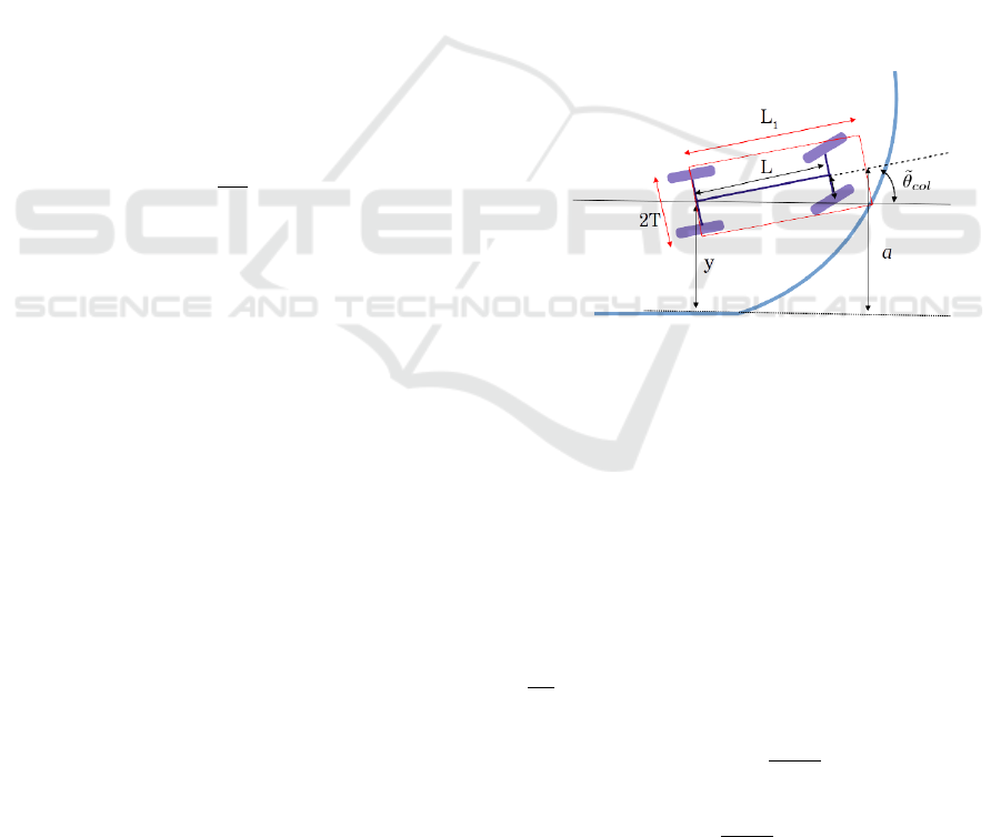
4.1 Limitation of the Robot Orientation

In Fig. 3, one can observe that when regulating a de-

sired lateral distance, the front of the robot may touch

the structure when this latter proposes important cur-

vatures.

Figure 3: Case of collision while the robot is well regulated.

In such a conﬁguration, the robot must overstep

the nominal regulation laws and turn in order to avoid

collisions. It is possible to compute the maximal ad-

missible orientation of the robot to avoid the collision.

This angle, denoted

col

, may be geometrically de-

ﬁned by:

y = a + T + L

sin

col

, (25)

with T the half-track of the robot and a the distance

between the tangent at the trajectory and the impact

point. If we consider that the trajectory is locally cir-

cular (such as suggested in Fig. 3), with a radius of

c(s)

, this distance a may be approximated by the fol-

lowing expression:

a =

1−cosγ

c(s)

, (26)

with γ = arctan(L

c(s)). The expression (25) exists

under the condition |

y−V −a

| < 1, which means that

the front of the robot stays on the good side of the

structure, which is assumed to be the case in practice.

ICINCO 2019 - 16th International Conference on Informatics in Control, Automation and Robotics

108

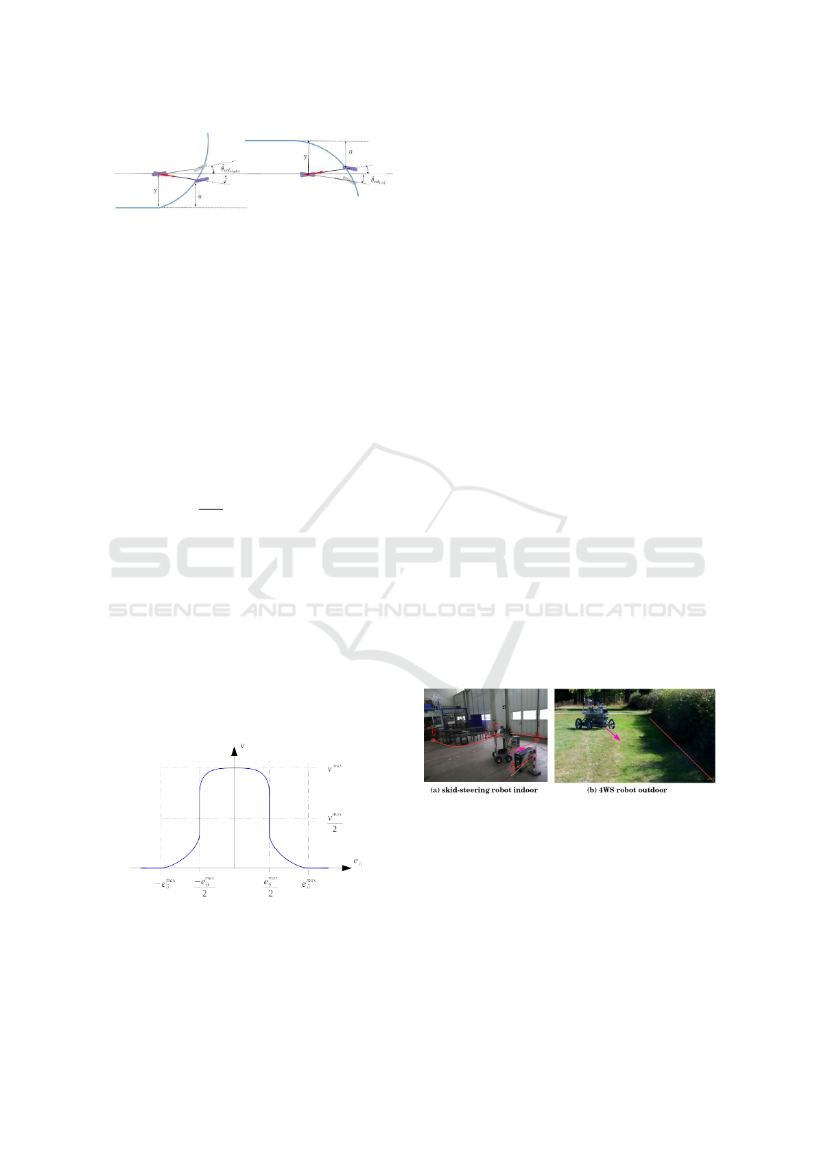
Figure 4: Case of collision on the right and the left.

Since the structure to be followed can be located

on the right or on the left of the robot,

col

has two

possible values denoted

col

right

and

col

le f t

, depend-

ing on the side where the structure is, as depicted in

Fig. 4. As soon as these two limits are known, an ad-

vantage of the proposed backstepping approach lies

in the fact that the desired orientation of the robot

computed by the control law (6) can be bounded. In

the following, the limits are computed in real time and

the targeted orientation is deﬁned such as:

θ =







ξ if

col

right

< ξ <

col

le f t

col

le f t

if ξ >

col

le f t

col

right

if ξ <

col

right

(27)

with ξ = arctan





− δ

, such as deﬁned by (6).

4.2 Limitation of the Robot Speed

In order to ensure an accurate edge tracking, it is rel-

evant to take the actuator settling time into account.

Indeed, the major consequences of this parameter are

overshoots on the tracking error. To limit this phe-

nomenon, it has been chosen to link the linear speed

of the robot with its angular deviation with respect to

the edge (i.e. v = f (

θ −

) = f (e

)). A proﬁle, such

as the one illustrated in Fig. 5 can be considered. This

permits to adjust the linear speed of the robot when a

tricky and narrow edge following appears.

Figure 5: Dependency between the linear speed and the

robot angular deviation.

Indeed, this proﬁle is deﬁned thanks to two pa-

rameters: the maximum linear speed of the robot v

max

and a threshold in the orientation error e

chosen in

advance. As long as the absolute value of the error is

lower than a threshold, the linear speed of the robot is

positive. It decreases when the orientation error e

ap-

proaches the threshold angle and is null beyond. This

is applied on a skid-steering robot, since it can turn on

itself, and then resume its motion to ensure a relevant

structure following.

5 EXPERIMENTAL RESULTS

5.1 Experimental Testbed

The proposed control framework has been tested on

two robots in two different conditions, depicted in

Fig. 6:

• a skid-steering mobile robot, moving in indoor

conditions, and following several kinds of struc-

ture (box, wall, shelves), such as depicted in

Fig. 6(a). It is a 25kg electric robot with a wheel-

base of 0.6m. The Lidar is setlled at 0.8m from

the rear wheel;

• a four-wheel-steering mobile robot moving in off-

road conditions, following a row of trees (see

Fig. 6(b)). This is a 520kg robot with a 1.2m-

wheelbase. The Lidar is situated at 1.8m from the

middle of the rear axle.

Both of the robot are equipped with a Sick-LMS laser.

The structures to be followed, quite different, are de-

picted by red lines in Fig. 6, reﬂecting some harsh

curvature in indoor conditions and an almost straight

line structure in outdoor conditions. The running di-

rection is depicted by the pink arrow.

Figure 6: Robots during the experiments: (a) indoor skid-

steering mobile robot (b) outdoor four-wheel-steering mo-

bile robot.

The structures are detected relying on the algo-

rithm described in Figure 7. It permits to obtain a

relevant and smooth trajectory in both indoor and out-

door environments.

A Generic Control Framework for Mobile Robots Edge Following

109

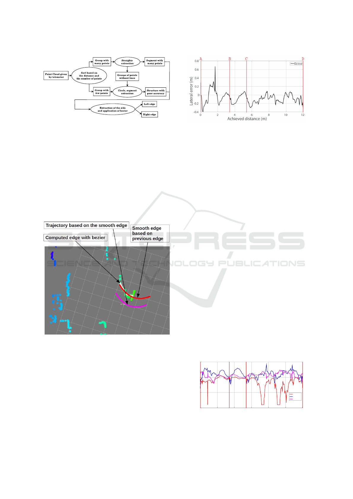
Figure 7: Algorithm to estimate surrounding structures.

5.2 Skid-steering Robot in Indoor

Conditions

The ﬁrst experiment proposed in this paper consists

in an indoor structure following by the skid-steering

mobile robot shown in Fig. 6(a). During this test, the

robot follows a box on the right and then a box on the

left (from A to B), it then follows a large door (from B

to C), and shelf legs arranged in circle (from C to D).

Fig. 8 shows a snapshot of the structure detection and

the trajectory generated when the robot is following

the structure from C to D.

Figure 8: Trajectory generation during the structure follow-

ing in indoor conditions between C and D.

One can see in Fig. 8 the laser impact points on the

shelf legs in green, the points of interest generated in

white and the computed trajectory in red, using a sec-

ond order polynomial curve ﬁtting. The objective is

to follow the various structures with a desired lateral

deviation y

of 1m. The results related to the track-

ing error e

during this ﬁrst experiment are depicted

in Fig. 9. In this ﬁgure, one can see that when the

trajectory is achievable, the error converges and stays

around 0, with an accuracy of few centimeters.

This is especially the case when the robot is fol-

Figure 9: Result of the tracking error during the indoor ex-

periment.

lowing the part between C and D, since the curvature

stays quite low. In contrast, one can see important

deviations:

• at curvilinear abscissa 1m, when the robot

switches from the box on the right to the one on

the left;

• around points B and C, when the robot has to fol-

low high curvatures.

At these points, a discontinuity in the edge occurs. As

a result, these errors are linked to the modiﬁcation of

the shape to be followed and can then be viewed as an

initial error, canceled after the robot has moved.

Moreover, when the robot faces high curvatures, there

is a risk of collisions and the desired orientation

bounded by

col

right

, as it is shown in Fig. 10. In this

ﬁgure, the desired orientation

is reported in ma-

genta and compared with the actual one

θ in blue. The

minimal admissible orientation

col

right

is reported in

red (maximal in terms of absolute value). One can

then see that at each large deviation (just after points

B and C), when the robot has to achieve an almost

◦

turn, the minimal value bounds the desired value

to avoid collisions. As a result, the tracking error is

not correctly regulated since the minimal value is im-

posed instead of the one required to reach the desired

lateral deviation y

. The same phenomenon can be

observed around curvilinear abscissa 9m. Elsewhere,

the minimal acceptable value stays far from the de-

sired one and may reach 90

◦

, which is the default

value.

Achieved distance (m)

0 2 4 6 8 10 12

Angular error (°)

-100

-50

Minimal

Actual

Desired

Figure 10: Desired, actual, and minimal orientations during

the indoor experiment.

ICINCO 2019 - 16th International Conference on Informatics in Control, Automation and Robotics

110

5.3 4WS Robot in Outdoor Conditions

The second experiment proposed in this paper con-

sists in an outdoor structure following by a four-

wheel-steering robot. Here, the objective is to follow

a row of trees such as depicted in Fig. 6(b), with a

desired distance of 1.5m and the robot parallel to this

structure (i.e.

= 0). In these conditions, the struc-

ture is almost straight. As it can be seen in Fig. 11,

the trajectory generated (in red) is indeed nearly con-

sidered as a straight line, even if the impact points of

the laser (in yellow) are quite noisy.

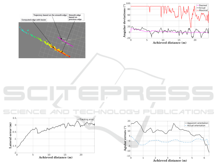
Figure 11: Trajectory generation during the structure fol-

lowing in outdoor conditions.

Thanks to the generation of the trajectory, the

robot is able to follow accurately the row of trees,

as illustrated by the tracking error shown in Fig. 12.

One can see that after the initialization phase, the er-

ror converges to zero and remains then close to this

value. One can also notice that the obtained accuraccy

is in the order of few centimetres.

Figure 12: Result of the tracking error during the outdoor

experiment.

This convergence is obtained thanks to the de-

sired orientation control proposed in this paper. The

desired orientation

is illustrated in Fig.13 in ma-

genta. The maximal admissible angle (the robot fol-

lows on the left), depicted in red in this ﬁgure, stays

far from the desired orientation, and does not disturb

in this case the accuracy of the tracking. One can

nevertheless see that this maximal orientation logi-

cally decreases, as soon as the robot comes closer

and closer from the actual structure. Since the de-

sired distance has been set to 1.5m (y

=1.5m) and

the half-track of the robot is equal to 0.6m, the robot

rear left wheel could collide the trees if the lateral er-

ror reaches 0.9m. This can be illustrated at curvilinear

18m, where the maximal admissible angle is close to

the actual one, as depicted in Fig. 13.

The desired orientation is compared to the orien-

tation

θ + δ

which is the variable actually con-

trolled for a 4WS robot (as detailed in section 3.3)

and illustrated in black. Despite some disturbances,

one can see a good correlation that allows to obtain

the satisfactory lateral position regulation illustrated

in Fig. 12.

Figure 13: Desired, actual, and maximal orientations dur-

ing the outdoor experiment.

It can also be veriﬁed that the rear steering law

allows to keep the robot parallel to the structure, as

desired (since

= 0). This can be particularly em-

phasized when focusing on the initialization phase of

the tracking (before the settling distance of 6m has

been reached). Fig. 14 compares the orientation

in black, and the actual one

θ in blue, from 0m to 6m.

Since the desired orientation

stays below 15

◦

, the

desired actual angle

is null, as ﬁgured out by the

relationship (24).

Figure 14: Comparison between

and the actual orienta-

tion

θ.

Thanks to control laws (22), the actual orientation

θ, whose initial value is 5

◦

converges and stays close

to zero, while the rear steering angle permits to con-

verge to a null tracking error. This point is particularly

important when considering agricultural tasks.

6 CONCLUSION

In this paper, a generic control algorithm for track-

ing accurately a structure at a desired distance is pro-

posed, based on an edge detection by a Lidar. It per-

A Generic Control Framework for Mobile Robots Edge Following

111

mits to address in a common framework, several kinds

of mobile robots, thanks to a backstepping approach.

A desired orientation is ﬁrst computed, allowing the

robot to converge to the desired distance from the

structure to be followed, whatever its conﬁguration

(skid-steering, car-like, or four-wheel-steering). This

is achieved using the derivative with respect to curvi-

linear distance, in order to have a behaviour which

is independent from the velocity. Beyond the con-

vergence of the lateral error, this ﬁrst step also per-

mits to detect and avoid collisions, by considering

the minimal and maximal admissible orientation, in-

side the motion control framework. Moreover, this

desired orientation is also used to compute a speed

limitation for skid-steering mobile robots, allowing

to achieve harsh manoeuvres. The second step con-

sists in the regulation of the orientation of the robot

to the desired one computed in the ﬁrst step. For

skid-steering robots, this is achieved relying on a

model with derivatives w.r.t. time, allowing them

to rotate even with a null longitudinal speed in or-

der to enhance the manoeuvrability. For four-wheel-

steering mobile robots (and consequently car-like mo-

bile robots), a strategy based on the curvilinear ab-

scissa is proposed, adding two steps in the approach.

The front steering angle is ﬁrst controlled to impose

that the orientation

(robot orientation increased by

the rear steering angle) converges to the desired one

and next the rear steering angle regulates the actual

robot orientation to increase the manoeuvrability or to

ensure the parallelism of the robot with respect to the

structure to be followed, depending on the situation.

Such an approach permits to regulate independently

the position and the orientation of the robot.

The effectiveness of the proposed algorithm has

been investigated through full scale experiments,

showing its robustness and efﬁciency in various con-

ditions, with different kinds of structures to be fol-

lowed (indoor furnitures and vegetations) and with

several kinds of robots. In particular, this algo-

rithm has been successfully tested on a 25-kg skid-

steering robot and on a 520-kg four-wheel-steering

robot, showing the generality of the proposed con-

trol law(s). This opens the way to achieve fully au-

tonomous agricultural tasks, especially in orchard or

vineyard, for spraying application. A new robot, able

to carry out an automated sprayer is indeed under de-

velopment to test such an approach in fully working

conditions.

ACKNOWLEDGMENT

This work has been sponsored by the French Na-

tional Research Agency under the grant number

ANR-14-CE27-0004 attributed to Adap2E project

(adap2e.irstea.fr). It has also been sponsored by

the French government research program ”Investisse-

ments d’Avenir” through the IDEX-ISITE initiative

16-IDEX-0001 (CAP 20-25), the IMobS3 Labora-

tory of Excellence (ANR-10-LABX-16-01) and the

RobotEx Equipment of Excellence (ANR-10-EQPX-

44). This research was also ﬁnanced by the European

Union through the Regional Competitiveness and

Employment program -2014-2020- (ERDF – AURA

region) and by the AURA region.

REFERENCES

Astrand, B. and Baerveldt, A.-J. (2005). A vision based

row-following system for agricultural ﬁeld machinery.

Mechatronics, 15(2):251 – 269.

Bayar, G., Bergerman, M., Koku, A. B., and Konukseven,

E. I. (2015). Localization and control of an au-

tonomous orchard vehicle. Computers and Electron-

ics in Agriculture, 115:118 – 128.

Bergerman, M., Billingsley, J., Reid, J., and Van Henten,

E. (2016). Robotics in Agriculture and Forestry. In

Springer Handbook of Robotics, pages 1463–1492.

Springer International Publishing.

Blackmore, S. (2016). Towards robotic agriculture. In SPIE

Commercial+ Scientiﬁc Sensing and Imaging, pages

986603–986603. International Society for Optics and

Photonics.

Cariou, C., Lenain, R., Thuilot, B., and Martinet, P. (2010).

Autonomous maneuver of a farm vehicle with a trailed

implement: motion planner and lateral-longitudinal

controllers. In IEEE International Conference on,

Robotics and Automation (ICRA), pages 3819–3824.

Cherubini, A. and Chaumette, F. (2013). Visual naviga-

tion of a mobile robot with laser-based collision avoid-

ance. The International Journal of Robotics Research,

32(2):189–205.

D’Andr

ea-Novel, B., Campion, G., and Bastin, G. (1995).

Control of nonholonomic wheeled mobile robots by

state feedback linearization. The International journal

of robotics research, 14(6):543–559.

Deremetz, M., Lenain, R., Couvent, A., Cariou, C., and

Thuilot, B. (2017). Path tracking of a four-wheel steer-

ing mobile robot: A robust off-road parallel steering

strategy. In European Conference on Mobile Robots

(ECMR), pages 1–7.

Lenain, R., Deremetz, M., Braconnier, J.-B., Thuilot, B.,

and Rousseau, V. (2017). Robust sideslip angles ob-

server for accurate off-road path tracking control. Ad-

vanced Robotics, 31(9):453–467.

Marmoiton, F. and Slade, M. (2016). Toward Smart Au-

tonomous Cars. In Intelligent Transportation Systems:

ICINCO 2019 - 16th International Conference on Informatics in Control, Automation and Robotics

112

From Good Practices to Standards, pages 84–109.

CRC Press.

Samson, C., Morin, P., and Lenain, R. (2016). Modeling

and control of wheeled mobile robots. In Springer

Handbook of Robotics, pages 1235–1266. Springer.

Tourrette, T., Lenain, R., Rouveure, R., and Solatges, T.

(2017). Tracking footprints for agricultural applica-

tions: a low cost lidar approach. In IEEE/RSJ Interna-

tional Conference on Intelligent Robots and Systems:

Agri-Food Robotics Workshop.

A Generic Control Framework for Mobile Robots Edge Following

113