
Improving Indoor Positioning via Machine Learning
Aigerim Mussina
a
and Sanzhar Aubakirov
b
Department of Computer Science, al-Farabi Kazakh National University, Almaty, Kazakhstan
Keywords:
Bluetooth Low Energy, Indoor Positioning, RSSI, Machine Learning, Support Vector Machine.
Abstract:
The problem of real time location system is of current interest. Cities are growing up and buildings become
more complex and large. In this paper we will describe the indoor positioning issue on the example of user
tracking, while using the Bluetooth Low Energy technology and received signal strength indicator(RSSI). We
experimented and compared our simple hand-crafted rules with the following machine learning algorithms:
Naive Bayes and Support Vector Machine. The goal was to identify actual position of active label among three
possible statuses and achieve maximum accuracy. Finally, we achieved accuracy of 0.95.
1 INTRODUCTION
The problem of positioning in indoor space is rele-
vant and include many complex substasks. The main
problem that will be discussed in this paper is the
user tracking in a defined environment. We are in-
terested in the detection of signal source’s position
among three distinguished parts of the building en-
trance: outside of the building, in vestibule and in-
side of the building. Our goal is to estimate and
compare machine learning algorithms and our hand-
crafted rules in position detection.
Main items of our indoor positioning system are
as follows: • base station - device that listen for ac-
tive label advertising and send its rssi to the desktop
server software; • active label - Beacon that act as
BLE advertiser; • server software calulate the active
label position and save data to database
We are using Bluetooth Low Energy(BLE) com-
patible devices, Beacons, as active labels because of
their sufficiently small size, low battery consumption,
lower cost. Beacon is based on Bluetooth low en-
ergy proximity sensing by transmitting a universally
unique identifier picked up by a compatible app or
operating system. Position calculation based on the
RSSI values. Since beacon transmit radio waves,
RSSI value oscillate influenced by absorption, inter-
ference and diffraction effects. In this case, there
should be implemented special filter to make RSSI
amplitude lower.
a
https://orcid.org/0000-0002-7043-0810
b
https://orcid.org/0000-0002-8416-527X
2 RELATED WORKS
In the work (Mussina and Aubakirov, 2018), we have
estimated the RSSI filtering algorithms, such as: me-
dian, mode, single direction outlier removal, shifting
and feedback filtering.
• Mode method counts occurrences of each RSSI
value and finds RSSI with maximum occurrences.
• Median method sorts all RSSI values at first, then
it chooses RSSI in the middle of the list.
• SDOR presented in work (Chai et al., 2016)
uses ten recent RSSI values to calculate thresh-
old. Their mean (rssi
mean
) and standard deviation
(rssi
std
) of these ten RSSI are calculated. Any
RSSI that is below (rssi
mean
− 2 ∗ rssi
std
) is re-
moved from the stored RSSI. Then the average
value of the remaining RSSI, rssi
p
, is the pre-
processed RSSI and used in next calculations.
• Feedback filtering based on idea that RSSI of
round n-1 affect RSSI of round n, see formula (1).
The average value of all calculated RSSI is corre-
sponding to smoothed RSSI value. See example
in figure 1.
• Shifting filtering based on the same idea as a feed-
back filtering except the definition of a round. In
shifting filtering, round is a period of 3 seconds.
During round system gets number of RSSI, and if
it is first round it calculates the average value of
all received RSSI, else it use formula (1), where
RSSI
n
is received RSSI and RSSI
n−1
is smoothed
average value of previous round. The average
value of all calculated RSSI is corresponding to
190
Mussina, A. and Aubakirov, S.
Improving Indoor Positioning via Machine Learning.
DOI: 10.5220/0007916601900195
In Proceedings of the 8th International Conference on Data Science, Technology and Applications (DATA 2019), pages 190-195
ISBN: 978-989-758-377-3
Copyright
c
2019 by SCITEPRESS – Science and Technology Publications, Lda. All rights reserved
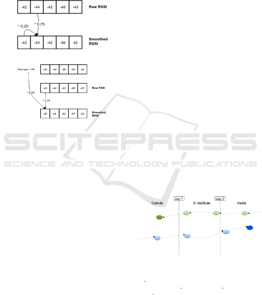
smoothed RSSI value of round n. See example in
figure 2.
RSSI = α ∗RSSI
n
+ (1 − α) ∗ RSSI
n−1
(1)
, where α is a coefficient and equal to 0.75.
Figure 1: Feedback filtering example.
Figure 2: Shifting filtering example.
Comparison of RSSI filtering algorithms shows
feedback and shifting as the best filter among pre-
sented. In further calculations we used feedback fil-
tering.
The machine and deep learning have been used in
localization problem solving during last years. The
work (Ibrahim et al., 2018) described the deep learn-
ing approach on the example of Convolutional Neu-
ral Networks. The main difference of (Ibrahim et al.,
2018) research among other is in a usage of RSS time-
series to reduce the noise. Authors used public dataset
(Torres-Sospedra et al., 2014) focused on WLAN
fingerprint-based indoor localization technique. It
consists of 529 features that can describe in what
building, floor and position user with smart phone is
located. Authors achieved accuracy of 100% in pre-
diction of building and floor. For estimation of coor-
dinates prediction the mean error was used. Task and
experiment of current article is specific and we need
to collect our own dataset for training and testing the
models. We also rely on the idea that series of RSSI
among time should produce better results.
Convolutional Neural Networks also im-
plemeneted in (Iqbal et al., 2017). The purpose
of real time location system in (Iqbal et al., 2017)
was to monitor clinical workflow and track patients.
Authors combined CNN with Artificial Neural
Network (ANN) and got better accuracy than with
single CNNs.
Together with Neural Networks, work (Qathrady
and Helmy, 2017) examine the machine learning tech-
niques such as Linear Regression, Decision Trees
and Random Forests. Authors made deep research
on transmission power value, TX power, which im-
proved classification accuracy.
The choice of machine learning algorithms was
based on the work (Ahmadi and Bouallegue, 2017),
which shows a survey on machine learning tech-
niques for localization using RSSI. The conclusion of
the article presented perfomance evaluation of Naive
Bayes, Decision Tree, Support Vector Machines, Ar-
tificial Neural Network and k Nearest Neighbors tech-
niques. The Naive Bayes approach showed lower lo-
calization error with Decision Tree and Support Vec-
tor Machines. We suppose that solution of the local-
ization problem should be simple. Therefore, hand-
crafted rules will be compared with Naive Bayes and
Support Vector Machines techniques.
Finally we will try to compare localization accu-
racy between our system and some systems presented
in mentioned above papers.
3 METHODS
The main task was to identify active label position
during its path from outside of the building to in-
side and vice versa. We have many active labels that
go between two base stations placed at the edges of
the vestibule, figure 3. In our experiments we avoid
smartphones, since work (Mussina and Aubakirov,
2018) shows smartphone make RTLS dependent on
its signal receiving capability.
Figure 3: Experiment visualization.
Main statuses for active labels are INSIDE,
IN VESTIBULE and OUTSIDE. Secondary sta-
tuses are LOST INSIDE, LOST OUTSIDE and
LOST UNKNOWN. Secondary statuses are deter-
mined by simple rules, based on received signal or
previous status:
• If base station one, esp1 from figure 3, received
signal and base station two, esp2 from figure 3,
Improving Indoor Positioning via Machine Learning
191
did not receive signal, then active label is lost
somewhere outside of the building.
• If base station one did not receive signal and base
station two received signal, then active label is lost
somewhere inside.
• If no base station received signal, then determine
by previous status.
– Active label is lost inside, if previous status was
INSIDE.
– Active label is lost outside, if previous status
was OUTSIDE.
– Active label status is LOST UNKNOWN, if
previous status was IN VESTIBULE.
The main research was directed at the determining
status, when both base station received signals from
active labels. We tried two approaches: hand-crafted
rules and machine learning.
3.1 Dataset
At first, let us introduce some common definitions of
classification applicable to our problem, to make fur-
ther explanations more readable and understandable.
Classification is a task of assigning a target value
t
i
∈ T to each vector hd
1
, d
2
, ..., d
M
i ∈ D, where D is
a domain of features, M is a total number of features
and T is a target values array. Features in our case are
RSSIs from two base stations and target values are
T = {INSIDE, IN V EST IBULE, OUT SIDE}.
Initially domain vector has size M = 2, D =
{RSSI
1
, RSSI
2
}. However, after first test we guessed
that machine learning can be improved by increas-
ing RSSI vector size M. Finally, we have exper-
imented with different vector’s sizes. For exam-
ple, if we would like to take into account 3 last
RSSIs from both base stations, then M = 6, D =
{RSSI
1,1
, RSSI
1,2
, RSSI
1,3
, RSSI
2,1
, RSSI
2,2
, RSSI
2,3
}
In the subsection 4.2 we will show work of ma-
chine learning approach on different RSSI vectors.
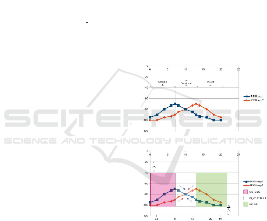
3.2 Hand-crafted Rules
In theory, graph with RSSI from both base station
and one active label should look like in figure 4.
It is obvious that esp1’s RSSI will be higher than
esp2’s RSSI, if Beacon, active label, will be out-
side. Similarly, esp2’s RSSI will be higher than
esp1’s RSSI, if Beacon will be inside. Determin-
ing Beacon’s status in vestibule is the most diffi-
cult part of the research. In vestibule active label
could be closer to esp1 or esp2, our hand-crafted
rule based on the direction of pair of RSSIs, as de-
picted in figure 5. The domain vector looks like D =
{RSSI
1,1
, RSSI
1,2
, RSSI
2,1
, RSSI
2,2
}. For example, if
domain vector look like D = {−76, −73, −80, −90},
then active label is in vestibule. All rules can work, if
base stations are the same and there are no obstacles
between Beacon and stations. Conditions for statuses
look as follow:
1. INSIDE
• RSSI from esp1 lower than RSSI from esp2
2. IN VESTIBULE
• RSSI from esp1 and esp2 are equal
• RSSI values from esp1 decrease and RSSI from
esp2 increase, figure 5 upper X-axis
• RSSI values from esp1 increase and RSSI from
esp2 decrease, figure 5 lower X-axis
3. OUTSIDE
• RSSI from esp1 greater than RSSI from esp2
Figure 4: RSSI from both base station in theory.
Figure 5: RSSI with directions.
3.3 Machine Learning Algorithms
We chose Naive bayes and SVMs algorithms for our
research. For both approaches we used Orange li-
brary. The Naive Bayes(NB) is a supervised learning
algorithm that can be used with continuous variables.
NB technique based on the Bayes’ theorem with the
feature independence assumption. This independence
plays role during calculation of conditional probabil-
ity, formula 2.
DATA 2019 - 8th International Conference on Data Science, Technology and Applications
192
P(c|x) =
P(X|c)P(c)
P(x)
(2)
, where P(c|x) - posterior probability of given class
value c and feature value x, P(c) - class prior proba-
bility, P(x|c) - likelihood, probability of x with given
c, P(x) - predictor prior probability.
Support Vector Machine(SVM) classification ap-
proach is another supervised algorithm that construct
optimal plane, hyperplane, separating smaples by
their classes. SVM defines the classification function
as in formula 3.
f (x) = sign(hw, xi + b) (3)
, where h, i is the scalar product, w is the normal vec-
tor to the separating hyperplane, b is an auxiliary pa-
rameter.
4 EXPERIMENTS AND
DISCUSSION
Experiments consists of two main parts: data collec-
tion and data processing.
4.1 Data Collection
At first, we needed to collect dataset with RSSI from
two base station and appropriate class, since machine
learning algorithms need sufficiently large dataset to
obtain model of prediction.
Assumptions:
• The base station performed by ESP-WROOM-
32 devices. ESP-WROOM-32 is an Espressif’s
miniature high-performance, combined Wi-Fi +
Bluetooth + BLE module, designed for a wide
range of applications. It is made on the basis of
the popular dual-core chipset ESP32. Device is
small, cheap and easy programmable on C lan-
guage.
• Size of environment was 18.35m x 3m. Base
stations are located at the distance of 2.35 me-
ters at the center, where vestibule supposed to lo-
cate. Imagined outside and inside area was of 8m
length.
• The active label performed by iTAG product
based on the Bluetooth 4.0 version. iTAG is a kind
of Bluetooth Low-energy product. It is also cheap
and sufficiently small to go with it.
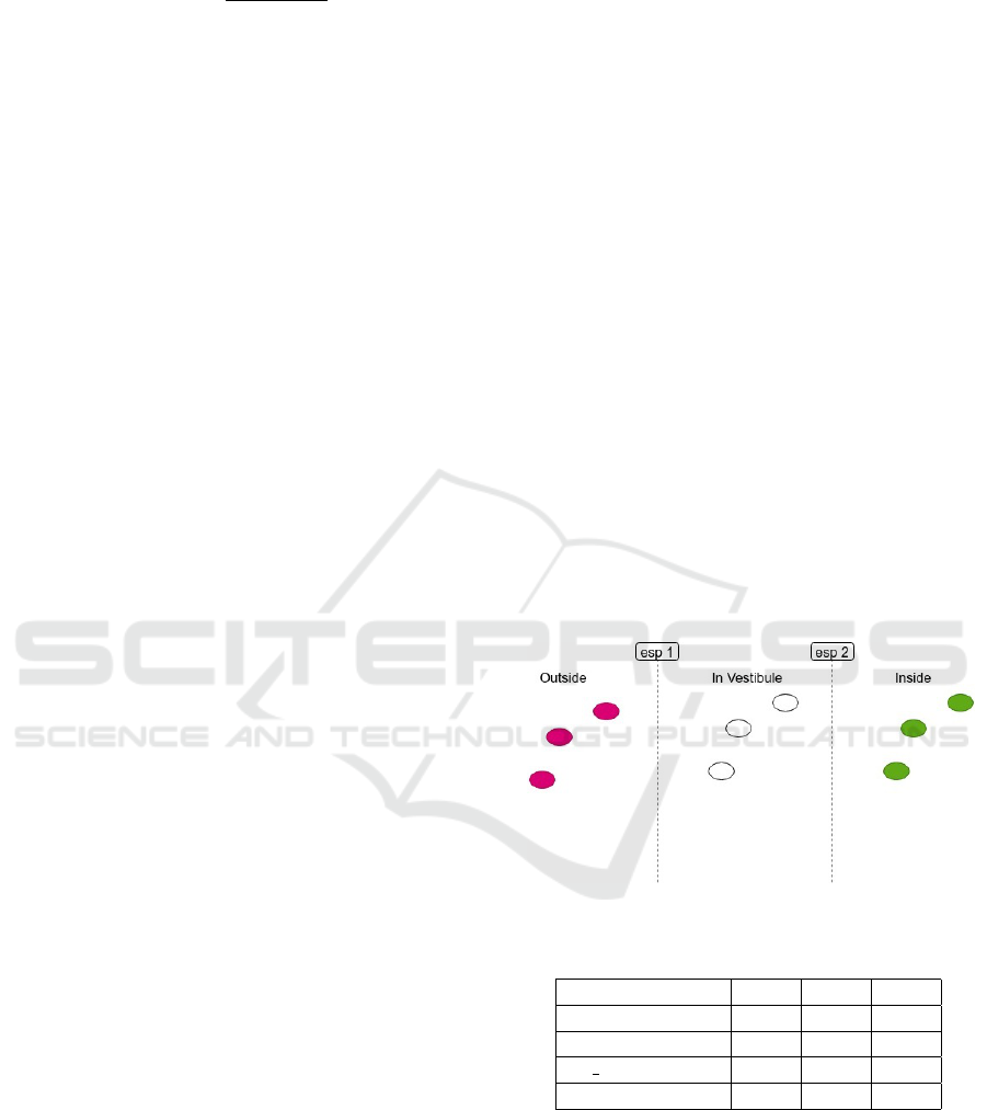
• iTAG devices devided to three group by color:
pink, white and green. Each group located at the
appropriate class position, see figure 6.
• During 20 minutes, trainee walk with iTAG in dif-
ferent directions within their class position such
that iTAGs are not stand still.
• Environment is Non Line of Sight Chan-
nel(NLOS). NLOS occurs when there are obstruc-
tions between the source and receivers, which
can cause large positive biases in the correspond-
ing distance information (Zekavat and Buehrer,
2012). Obstacles such as human body and all ac-
tivated iTAG devices are presented.
Base station scan for signals from iTAG devices
every 100ms among 1 second. After 1 second, base
station sends collected signals’ information to the
software server. The signal’s information consists of
base station’s id, iTAG address and RSSI. Server soft-
ware accept data, filter RSSI among each received
iTAG and save data to database. Also it saves iTAG
address to the list of active devices. Another soft-
ware thread reads each second RSSIs from database
for iTAG devices which are in the list of active de-
vices. Thread reads from database the last saved
within 5 seconds RSSI from both base stations and
save new sample to database. After saving thread re-
moves iTAG from active device list.
Collected dataset shown in table 1.
Figure 6: Data collection.
Table 1: Dataset.
all train test
Dataset 9984 7988 1996
INSIDE 3165 2532 633
IN VESTIBULE 3423 2739 684
OUTSIDE 3396 2717 679
4.2 Data Processing
In subsection 3.1, we desribed classification domain
which is constructed as a series of RSSI by time. Pro-
ducing such domain vectors caused problem of find-
ing the exact size M of the domain vector D. Con-
sidering the velocity of human walk, which is 1.38
m/s, we assumed that it is needed to process RSSIs
Improving Indoor Positioning via Machine Learning
193
received at each second. During this experiments our
iTAG devices were not configured to pass exact num-
ber of signals per seconds. Analysis of dataset give us
that maximum number of received RSSI values from
one device during one second is four, but this num-
ber is not usual for our dataset. Usually we got two
or three RSSI values per second from each device.
For this research we will take into account vector size
from 1 to 4, as the absolute minimum and absolute
maximum numbers of RSSIs values that could be re-
ceived per second.
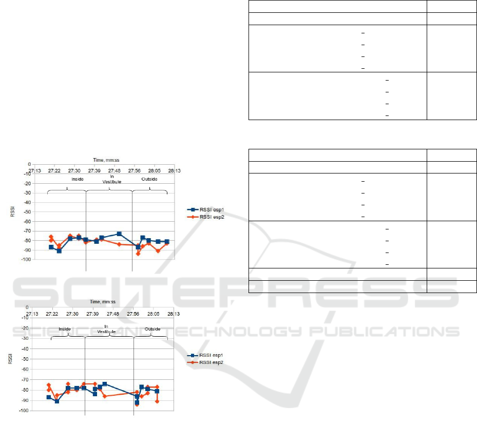
Subsection 3.2 described the view of RSSI from
two base station in theory. Results from the test were
different as expected. Figures 7 and 8 show RSSI fil-
tered and non-filtered respectively.
Figure 7: RSSI filtered.
Figure 8: RSSI non-filtered.
Filtered RSSI looks more reliable. In outside part
non-filtered RSSI from esp2 sometimes is greater than
RSSI from esp1, which is not correct in theory. Con-
trariwise, filtered RSSI from esp1 in outside part is
greater than from esp2, which is theoretically true.
We checked the assumption that machine learn-
ing approach could work better on non-filtered RSSI.
All approaches were estimated by accuracy. Table 2
shows accuracy for non-filtered RSSI.
Table 3 demonstrates the accuracy of examined
techniques that worked with filtered RSSI and at the
same time depicts the results of works (Iqbal et al.,
2017) mentioned as CNN+ANN and (Qathrady and
Helmy, 2017) mentioned as TX, for half a meter esti-
mation. Hand-crafted rules showed lowest prediction
Table 2: Accuracy of all examined approaches on non-
filtered RSSI.
Technique accuracy
Hand-crafted rules 0.5136
Naive Bayes, vector size = 1 0.6752
Naive Bayes, vector size = 2 0.760
Naive Bayes, vector size = 3 0.821
Naive Bayes, vector size = 4 0.838
Support Vector Machine, vector size = 1 0.6734
Support Vector Machine, vector size = 2 0.768
Support Vector Machine, vector size = 3 0.834
Support Vector Machine, vector size = 4 0.855
Table 3: Accuracy of all examined approaches.
Technique accuracy
Hand-crafted rules 0.5836
Naive Bayes, vector size = 1 0.739
Naive Bayes, vector size = 2 0.842
Naive Bayes, vector size = 3 0.883
Naive Bayes, vector size = 4 0.926
Support Vector Machine, vector size = 1 0.741
Support Vector Machine, vector size = 2 0.881
Support Vector Machine, vector size = 3 0.927
Support Vector Machine, vector size = 4 0.958
CNN+ANN 0.999
TX, half a meter 0.950
capability.
Machine learning algorithms showed better accu-
racy than hand-crafted rules. Mainly hand-crafted
rules can’t work with unstable RSSI values, unless
values will be fileterd sufficiently enough for rules.
Machine learning demonstrates better results on fil-
tered RSSI.
Comparing accuracy from table 2 and table 3 we
can conclude that filtereing has improved accuracy for
a little bit.
SVM approach on data with RSSI’s vector of
size 4 presented better result among our approaches.
Comparing with (Iqbal et al., 2017) and (Qathrady
and Helmy, 2017) it has lower accuracy. The rea-
son could be in training datasets, because (Iqbal et al.,
2017) has 5 times more base stations which lead to
more data and the (Qathrady and Helmy, 2017) had
1.8 million records of RSSI. Also estimation of TX
power approach was held in clear environment with
no obstacles. In future works we will consider deep
learning approach and try to increase performance by
Neural Networks.
DATA 2019 - 8th International Conference on Data Science, Technology and Applications
194

5 CONCLUSIONS
We have used only two classification algorithms,
Naive Bayes and Support Vector Machine, that is very
small number. However, this research shows that ma-
chine learning is applicable for localization problem
and it is more effective than hand-crafted rules. Also
classification approach works better on filtered RSSI
and with more RSSI-features in dataset. In future
we will look for better filtering algorithm. Our next
research goals are experiment with bigger dataset,
compare filtration and classification algorithms within
this experiment of entry/exit, implement Neural Net-
works. After tests we got the assumption, that classifi-
cation may produce better results if we combine ma-
chine learning algorithms results with majority rule.
The main part in machine learning process is dataset
collection, which is very laborious process, that must
be clear and accurate. We will experiment with time
of scanning and RSSI receiving time matching be-
tween two base station. Finally, machine learning and
RSSI filtering make user tracking problem sufficiently
solvable. We achieved accuracy of 95.8%.
6 COPYRIGHT FORM
The Author hereby grants to the publisher, i.e. Sci-
ence and Technology Publications, (SCITEPRESS)
Lda Consent to Publish and Transfer this Contribu-
tion.
ACKNOWLEDGEMENTS
This research was conducted in the ”Internet of
Things” laboratory with support at the ”Artificial In-
telligence and Big Data” department of the al-Farabi
Kazakh National University.
REFERENCES
Ahmadi, H. and Bouallegue, R. (2017). Exploiting machine
learning strategies and rssi for localization in wireless
sensor networks: A survey. In 2017 13th Interna-
tional Wireless Communications and Mobile Comput-
ing Conference (IWCMC), pages 1150–1154.
Chai, S., An, R., and Du, Z. (2016). An indoor positioning
algorithm using bluetooth low energy rssi.
Ibrahim, M., Torki, M., and Y. Elnainay, M. (2018). Cnn
based indoor localization using rss time-series.
Iqbal, Z., Luo, D., Henry, P., Kazemifar, S., Rozario, T.,
Yan, Y., Westover, K., Lu, W., Nguyen, D., Long, T.,
Wang, J., Choy, H., and Jiang, S. (2017). Accurate
real time localization tracking in a clinical environ-
ment using bluetooth low energy and deep learning.
PLOS ONE, 13.
Mussina, A. and Aubakirov, S. (2018). Rssi based bluetooth
low energy indoor positioning. In The IEEE 12th In-
ternational Conference on Application of Information
and Communication Technologies / AICT 2018, pages
301–304.
Qathrady, M. and Helmy, A. (2017). Improving ble distance
estimation and classification using tx power and ma-
chine learning: A comparative analysis. pages 79–83.
Torres-Sospedra, J., Montoliu, R., Mart
´
ınez-Us
´
o, A., Avari-
ento, J., J. Arnau, T., Benedito-Bordonau, M., and
Huerta, J. (2014). Ujiindoorloc: A new multi-building
and multi-floor database for wlan fingerprint-based in-
door localization problems.
Zekavat, R. and Buehrer, R. M. (2012). Source Localiza-
tion: Algorithms and Analysis, pages 25–66. IEEE.
Improving Indoor Positioning via Machine Learning
195
