Comparative Analysis of Store Clustering Techniques in the Retail

Industry

Kanika Agarwal, Prateek Jain and Mamta Rajnayak

Accenture Digital, Accenture Private Solution Limited., India

Keywords: Store Clustering, Self Organizing Maps, Gaussian Mixture Matrix, Fuzzy C-means.

Abstract: Many offline retailers in European Markets are currently exploring different store designs to address local

demands and to gain a competitive edge. There has been a significant demand in this industry to use analytics

as a key pillar to take store-centric informed strategic decisions. The main objective of this case study is to

propose a robust store clustering mechanism which will help the business to understand their stores better and

frame store-centric marketing strategies with an aim to maximize their revenues. This paper evaluates four

advance analytics-based clustering techniques namely: Hierarchical clustering, Self Organizing Maps,

Gaussian Mixture Matrix, and Fuzzy C-means These techniques are used for clustering offline stores of a

global retailer across four European markets. The results from these four techniques are compared and

presented in this paper.

1 INTRODUCTION

Over the last decade, there has been a steady growth

in the European retail market. Retailers have designed

different store designs across the markets to cater to

local customer preferences and to gain competitive

advantage. There has been a significant demand for

analytics in the market to drift from traditional

descriptive to more of a predictive/prescriptive

approach.

According to a report by Neilsen, there has been a

shift in the convenience store’s transaction and

purchase patterns. The store visit has increased,

however, spending per visit has decreased. There has

been a change in customer lifestyle, for instance,

people prefer fresh and healthy products nowadays.

Availability of contactless payment method, self-

checkouts also have a positive impact on store

footfall. Analyzing these factors would help the

retailer in maximizing profit and optimizing

inventory.

The retailers are concerned with the following

business problems.

1. How are the various stores performing? Which

stores have the maximum potential to grow?

2. What is the customer footfall? What is the

average spending per transaction?

3. What kinds of products are purchased the

most? Is it tobacco, coffee, grocery or any

other category?

4. What are the top performing manufacturers

and brands?

5. What type of customers visits the stores? What

are their preferences?

6. How much is the store responsive to

promotion such as discount coupons, meal

deal offers etc.?

7. How accessible is the store? Is parking facility

available or is the store well connected?

8. What is the store firmographics: store size,

store layout, store design?

This paper is designed to address these business

problems and propose a strategic point of view to

retailers with an end objective to be more profitable

and competitive in the market.

The retailer considered in this paper is operational

in many European countries such as Germany,

Netherland, Austria, Poland, United Kingdom,

Switzerland etc. It has more than 5000 store outlets

and millions of customer base across all the

geographies. It offers a wide range of product

portfolio: groceries, tobacco, drinks, fast food,

packaged food etc. This retail organisation wants to

leverage power of analytics and better understand

their retail store business with an aim to stay ahead of

Agarwal, K., Jain, P. and Rajnayak, M.

Comparative Analysis of Store Clustering Techniques in the Retail Industry.

DOI: 10.5220/0007917500650073

In Proceedings of the 8th International Conference on Data Science, Technology and Applications (DATA 2019), pages 65-73

ISBN: 978-989-758-377-3

its peers. To achieve this aim, it is important for this

organisation to better understand the markets in

which they are operating and have a personalised

local view of the retail stores within these markets.

Hence, store segmentation is proposed to cater to

these business requirements. Given the complexity of

data and market dynamics, it is imperative to apply

some sophisticated clustering techniques which

would address the limitations of traditional

techniques like K-mean and agglomerative

clustering.

This paper proposes the use of advance machine

learning techniques like Self Organizing Maps

(SOM), Gaussian Mixture Models (GMM), Fuzzy C-

means (FCM) for clustering offline stores of different

European markets. The results of these techniques are

also compared with results of legacy clustering

technique like hierarchical to prepare a comparative

analysis for each market.

This paper is structured as follows. Section 2

presents the related literature available in this domain.

Section 3 describes the different data sources,

variables and techniques used in the analysis. Section

4 presents the comparative results of the techniques

applied across different markets and the paper is

concluded in Section 5.

2 RELATED WORKS

Various algorithms have been proposed by

researchers relating to clustering applications for

retailers in the literature and results from clustering

have been presented.

Researchers have classified internet retail sites for

an e-commerce company. 35 observable internet

retail store’s attributes are used, and hierarchical

clustering technique is applied to classify store into

five distinct web catalog interface categories:

superstores, promotional stores, plain sales stores,

one-page stores, and product listings. The classified

online stores differ primarily on the three dimensions:

size, service offerings, and interface quality (Spiller

and Lohse, 2015).

Researchers analyze the data of a supermarket

chain which has 73 stores in Turkey. Data related to

stores such as store size, number of competitors

nearby, trade area demographics like distribution of

population by age, marital status are used for

conducting the segmentation. Hierarchical clustering

is applied, and effective target marketing strategy is

designed for each store segment (Bilgic, Kantardzic,

and Cakir, 2015).

Researchers have applied artificial neural

networks (ANNs) as an alternative means of

segmenting customers in retail space. Hopfield–

Kagmar (HK) clustering algorithm, an ANN

technique based on Hopfield networks, is compared

with K-means clustering algorithms. Purchase

behavior such as the total number of orders, days

since first purchase, the number of credit cards etc is

used for profiling the customers. The results indicate

that ANNs could be more useful to retailers for

segmentation because they provide more

homogeneous segmentation solution than K-means

clustering algorithms and are less sensitive to initial

starting conditions (Boone and Roehm, 2002).

Researchers have applied clustering techniques

namely K-means clustering, Mountain clustering, and

Subtractive clustering on the dataset for medical

diagnosis of heart disease. It is observed that K-means

overperformed in cases where many dimensions are

present. Mountain clustering is suitable only for

problems with two or three dimensions (Hammouda

and Karray, 2002).

Most of the papers have applied hard clustering

techniques like K-means and hierarchical. Most of

them have been used for customer segmentation

rather than for store segmentation. Even if there is

some research in the store segmentation space, it is

predominantly focused on online channel than the

traditional offline channel. To add further, the

attributes used for store clustering are mostly related

to firmographics, customer demographics or

competitor information. In this paper, store clustering

is performed for a retail organisation. Attributes

related to purchase pattern, transaction pattern,

customer behaviour, store dimensions are used for

clustering. Both hard clustering technique such as

hierarchical clustering and soft clustering techniques

such as Self Organizing Maps (SOM), Gaussian

Mixture Models (GMM), Fuzzy C-means (FCM) are

applied for clustering stores for four different

European markets. A comparative study on the results

derived from these different techniques for different

markets has been presented in this paper.

3 DATA AND METHODLOGY

The retailer considered is a UK based multinational

organization offering convenience retail services to

.consumers. The company operates through various

channels. Some of the stores are owned and operated

by the company itself, however, there are some which

are owned and operated by a franchise or a dealer.

DATA 2019 - 8th International Conference on Data Science, Technology and Applications

In this paper, data is analyzed for four different

European markets. The time frame considered for the

analysis is one year. The data sources used are

transaction data, product data, store data, loyalty data,

and competitor’s data. In transaction data, attributes

like transaction date, sales, quantity etc. are captured.

Attributes like product description, category

description, brand etc. are captured in the product

dataset. Dimensions like store size, location,

operating channel etc. are recorded in the store data.

Information related to purchase behavior of the

customers using the loyalty card, methods of

payments, discounts, point redemption etc. are

captured in the loyalty data. Competitor’s data

included the competitor’s pricing attributes. All the

datasets together have millions of transactions

encapsulating close to a hundred raw variables.

Table 1: Description of some of the variables captured in

the dataset.

Variable name Data type Description

Transaction id Varchar

Unique id associated

with each transaction.

Transaction

date

Time

stamp

Time at which

transaction is recorded.

Product id Varchar

Unique id the product

purchased.

Store id Varchar

Unique id of the store in

which the product is

sold.

Sales Numeric

Sales value of the

product.

Quantity Numeric

Quantity in which

product is sold.

Product

description

Varchar

Description of the

product sold.

Category

description

Varchar

Description of the

category the product

belonged to such as

tobacco, drinks etc.

Operating

channel

Varchar

Flag to identify id the

store owned by

company or not.

Location Varchar

Indicate if the store is

located centrally or if it

is in countryside.

3.1 Data Wrangling

To perform store clustering, the data must be

represented at a store level. So, after collating the

datasets, all the variables are rolled at a store level.

Depending on the nature of the variable, aggregation

methods like sum, count, max, min are applied. For

example, in the case of sales and quantity sum is

taken, however, in the case of transactions, a distinct

count is calculated. Many derived variables like

spending per category, average price, sales

corresponding to different months, week of the day

and time of the day are created. This led to the

creation of around 400 variables for each store. These

set of variables provide a holistic view of stores and

capture dimensions related to demographics,

firmographics, transaction pattern, purchase pattern

etc

In order to ensure that quality data is used for

clustering, a cleansing procedure is applied. The

process is as followed.

1. A univariate analysis is conducted to calculate

the percentile distributions (0.01, 0.05,

0.1,0.25, 0.5, 0.75, 0,9 ,0.95 ,0.99), count of

missing values etc.

2. As per the nature of the variable, missing value

imputation techniques like replacement with

mean/median/mode etc. are applied.

3. Variables with significant missing values are

excluded from the analysis.

4. Variables that showed less variability are also

removed.

5. The last step is the outlier treatment.

Depending on the distribution of the variable

the treatment is conducted. For some variables

percentile value is used to replace the

outlier at the upper end and similarly for

others, some other threshold is applied.

All the stores are not considered for analysis.

Only the stores that are owned by the company and

that are operational for more than 80% of the time

period are taken into account.

Conducting clustering on 400 variables is neither

efficient nor feasible. So, the next process is the

selection of relevant variables. To do this, the variable

clustering technique is applied. The package

ClustofVar in R is used for the same. Hierarchical

clustering technique is applied to club variables

strongly related to each other. The algorithm is

explained in detail in the section3.2.4. There is only

one difference, here the algorithm is applied to group

variables and in section 3.2.4 it is applied to group

stores. Once the variables are grouped into clusters, a

loading is attached to each variable. From each cluster

some variables are selected based on the loading

value and business inputs. Around 30 variables are

shortlisted to be used in the final clustering process.

Comparative Analysis of Store Clustering Techniques in the Retail Industry

3.2 Clustering Techniques

There are two kinds of clustering techniques: hard

clustering and soft clustering. In case of hard

clustering a data point belongs to only one cluster

However, in case of soft clustering, a data point has

the probability of belonging to all the clusters. K-

means and Hierarchical clustering fall under the hard

clustering classification while Self Organizing Maps

(SOM), Gaussian Mixture Models (GMM), Fuzzy C-

means (FCM) are a part of soft clustering

classification.

In this section, the hard clustering technique:

Hierarchical and soft clustering techniques: SOM,

GMM, FCM are explained in detail.

3.2.1 Self Organizing Maps

This is a type of artificial neural network which works

on the principle of reducing high dimensional data

into low dimensional space. The technique maintains

the spatial relationship between the data. The process

followed by SOM is as follows.

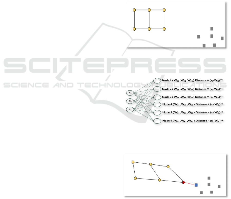
1. The very first step is the specification of grid

space as hexagonal or rectangular. For

example, grid space for 6 clusters could be

2x3, 1x6, 6x1 or 3x2. In figure1, it is

rectangular 2x3.

2. Once the grid is selected, each cluster/node in

the grid is assigned a random weight. The

dimension of a node is equivalent to the

number of variables in the data. For example,

in figure2, Node1 has 3 weight dimensions

corresponding to 3 variables (X

, X

) in the

data.

3. For each iteration, an observation is randomly

selected, and a distance metric is calculated

with respect to all the nodes as shown in

figure2.

4. The cluster with the minimum distance is

assigned to the observation.

5. As this happens, the whole grid moves closer

to the observations, as shown in figure3. The

movement is dependent on the learning rate

specified in the model.

6. Weights of the nodes are adjusted.

7. This completes an iteration for one

observation (Step 3-6).

8. In the next iteration, again one observation is

selected to pass through the above steps.

9. The process is repeated iteratively till all the

observations are assigned a cluster and a

convergence criterion is achieved.

The equation used for updating weight is as

follows.





1











































 (1)

where t is time step, W(t) is the weight at time t,

L is the leaning rate factor at time t, θ(t) is

neighbourhood function at time t.

The fine-tuning parameters for SOM are the cluster

number, the dimension of grid space, the learning rate

which determines the rate at which the node’s weights

are updated. For the analysis, the Kohonen package

in R is used. SOM is one of the techniques which is

very powerful when it comes to visualization of the

clusters across different dimensions.

Figure 1: This figure shows the grid 2x3 (on the left) and

the set of observations (on the right). (Source mentioned in

the references section).

Figure 2: This figure shows the calculation of distance for

observation with 3 dimensions. (Source mentioned in the

references section).

Figure 3: This figure shows how the grid moves when a

cluster is assigned to observation. (Source mentioned in the

references section).

DATA 2019 - 8th International Conference on Data Science, Technology and Applications

3.2.2 Gaussian Mixture Models (GMM)

This technique is a probabilistic approach to

clustering. GMM is a mixture of K Gaussian

component that means it is a weighted average of K

Gaussian (normal) distribution. The technique is

based on the Expectation Maximisation algorithm.

The technique works in the following way.

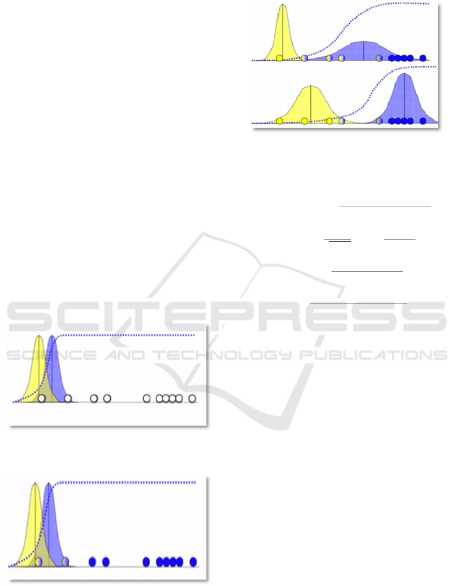
1. For each cluster, a mean and standard

deviation value is allocated. In figure4, there

are two clusters which have a normal

distribution with mean and standard deviation

as (µ

a )

,( µ

,σ

b) .

2. Then for each observation, the probability of

belonging to these 2 clusters is calculated

using equation2. In figure 5, the two different

colors per observation show the probability

attached to the corresponding distribution.

3. Using these probabilities, the mean and

standard deviation of the clusters are re-

estimated as shown in equation4 and

equation5.

4. The process keeps on repeating until

convergence is achieved. Figure 6 shows how

the final distribution changes over various

iterations.

Figure 4: This figure shows the initial distribution of two

clusters. (Source mentioned in the references section).

Figure 5: This figure shows the probability assigned to each

observation based on the parameters of the distribution.

(Source mentioned in the references section).

Figure 6: This figure shows the result after multiple

iterations. (Source mentioned in the references section).

The equations used in GMM are as follows.





  















⁄













⁄



















⁄



 (2)





 











exp



















 (3)

μ





















⋯















⋯



(4)

























⋯























⋯



(5)

Here x

is the ith observation, µ

is the mean of the

second cluster, σ

is the standard deviation of the

second cluster.

The optimal number of clusters is chosen based

on the Akaike Information Criterion and the Bayes

Information Criterion. Mclust package in R is used

for conducting the exercise.

3.2.3 Fuzzy C-Means (FCM)

This technique is like K-means, however, here every

observation has a degree of belonging to all the

clusters. The process for clustering is as follows.

1. Cluster centers are created randomly based on

the number of clusters.

2. Euclidean distance between the observations

and cluster centroids is calculated in this step.

3. Then, the membership matrix is generated,

using equation 6.

4. After this, the centroids are updated using

equation 7.

5. The last two steps are repeated until the

convergence criterion, as shown in equation 8

is achieved. The value of epsilon should be

between 0 and 1.

Comparative Analysis of Store Clustering Techniques in the Retail Industry

The equations are as follows.









∑



||







||

















(6)







∑















∑











(7)



















(8)

Where Uij

= membership of the ith data to the jth

cluster, m = fuzziness exponent, C = number of

clusters, c

= jth cluster centre , x

= ith observation ,

N = number of observations.

The fine-tuning parameters here are the number of

clusters and the fuzziness exponent “m” whose value

should be greater than one. For this exercise, fclust

package in R is applied.

3.2.4 Hierarchical Clustering

In hierarchical clustering, the bottom up clustering

approach is applied. The process applied is as

follows.

1. Each observation is considered as a single

cluster.

2. Then the distance between every pair of

observation is calculated and stored in a

distance matrix. The distance between cluster

can be calculated using complete linkage,

average linkage etc.

3. Pair closest to each other are merged together

and as a result, the number of clusters is

reduced by 1 in each step.

4. Step 2 and 3 are repeated until all the points

are a part of one big cluster.

At the end of the process, a dendrogram is created

as shown in figure7. This helps to identify the optimal

number of clusters. The package hclust in R is used

for the analysis.

Figure 7: This figure shows a dendrogram. The line depicts

the point at which dendrogram is cut.

4 IMPLEMENTATION AND

RESULTS

In section 3, the clustering modelling exercise is

discussed. This section describes the different steps

that are performed after the clustering modelling task

is completed.

4.1 Validation

Several iterations are performed, and many

parameters are considered to get the final iteration.

Some of the validation steps are as follows.

1. The number of clusters formed is decided

based on statistical as well as business inputs.

Some of the statistical techniques that are used

to identify the optimal set of clusters are

dendrograms, heatmaps etc. The number of

clusters formed lied in the range of 3-5

depending on the market and technique.

2. The minimum number of stores per cluster is

set to be at least 30.

3. The following parameters across iterations are

compared.

Table 1: Metrics compared.

Hierarchical Dunn Index, Silhoutte

coefficient

SOM Neighbour distance, Training

Progress

GMM Akaike Information Criterion,

Bayes Information Criterion

FCM Coefficient of Variation

4 All the clusters formed have some distinct

features that would ensure that stores within a

cluster are homogeneous and stores across

clusters are heterogeneous.

4.2 Profiling

There are two levels of profiling that are performed

during this exercise.

1. Basic profiling: In this, all the modelling vari-

ables that are used for clustering are considered

and their variations across the clusters are

captured. If the variables are numerical then

mean is considered and if the variables are

categorical then the frequency is considered.

2. Advance Profiling: In this, other variables

apart from modelling variables that are

relevant to the business are considered and

their variations across the clusters are captured

DATA 2019 - 8th International Conference on Data Science, Technology and Applications

in a similar way as described for basic

profiling. This helped in personifying the

clusters and capturing all the differentiated

attributes for each cluster. For instance, as

shown in figure 8, cluster 3 has the maximum

sales whereas cluster 4 has the minimum sales.

Cluster 1 has the maximum numbers of stores

and because of that, they have the maximum

number of the customer base as well. Spending

per transaction is another attribute that is used

to differentiate clusters. The spending per

transaction in cluster 1 is higher as compared to

others. Also, each cluster is dominant in at least

one of the categories. For example, category 1

has the maximum sales share for cluster 1

where as category6 is dominant in cluster 2.

This insight would help the category managers,

in better understanding and designing of the

strategies/promotions. Distribution of different

store designs within a cluster is also captured.

For instance, the stores of cluster 4 and 3,

majorly have Z layout whereas cluster 2 and 1

have mostly layout Y. This information helped

in better understanding of store attributes.

Figure 8: This figure shows the store profiling for one market using GMM.

KPIs Cluster1 Cluster2 Cluster3 Cluster4

Average

Value

Number of Sites 88 47 110 38 283

Share of Sites, % 31% 17% 39% 13%

Total Sales 2,518 m 968 m 3,449 m 681 m 1,904 m

Sales Share 33% 13% 45% 9%

Customer Count 501,200 230,345 631,134 239,234 400,478

Loyal Transactions/Overall Transactions (%) 44% 74% 56% 63%

Points Redeemed/Points Issue (%) 56% 61% 54% 72%

Transactions (Per Store) 165,130 157,152 173,600 335,215 178,514

Transactions (Per Month/Per Store) 14,056 13,125 14,524 28,338 15,025

Sales (Per Store) 3,602,804 2,643,445 3,139,645 5,792,097 3,369,966

Sales (Per Month/Per Store) 305,429 220,771 262,638 489,562 283,424

Units Per Transaction 2.5 2.2 2.9 2.5 2.6

Sales Per Transaction 21.8 16.8 18.1 17.3 18.9

Transactions (Per Store) 93 88 97 188

Transactions (Per Month/Per Store) 94 87 97 189

Sales (Per Store) 107 78 93 172

Sales (Per Month/Per Store) 108 78 93 173

Units Per Transaction 95 83 11

Sales Per Transaction 116 89 96 92

Category 1 111,565 16,992 20,806 107,820 64,296

Category 2 13,415 14,314 11,891 18,195 14,454

Category 3 21,930 11,645 15,668 83,616 33,215

Category 4 26,609 7,242 79,306 89,497 50,664

Category 5 21,669 16,307 18,651 50,751 26,844

Category 6 10,386 78,652 8,474 22,911 30,106

Category 7 2,713 1,842 2,025 7,974 3,638

Category 8 25,314 15,156 24,258 40,784 26,378

Category 1 48% 10% 11% 26%

Category 2 6% 9% 7% 4%

Category 3 9% 7% 9% 20%

Category 4 11% 4% 44% 21%

Category 5 9% 10% 10% 12%

Category 6 4% 49% 5% 5%

Category 7 1% 1% 1% 2%

Category 8 11% 9% 13% 10%

Store Size -Small 31% 25% 23% 23%

Store Size -Medium 34% 29% 44% 34%

Store Size -Large 35% 46% 33% 43%

Store Layout -X 23% 27% 25% 35%

Store Layout -Y 41% 50% 35% 24%

Store Layout -Z 36% 23% 40% 41%

Store KPIs

KPIs Per Store & Per Store/Month, Absolute Values

KPIs Per Store & Per Store/Month, Indices

Category Average Sales Per Site/Per Month

Category Average Sales Per Site/Per Month, % Share

Comparative Analysis of Store Clustering Techniques in the Retail Industry

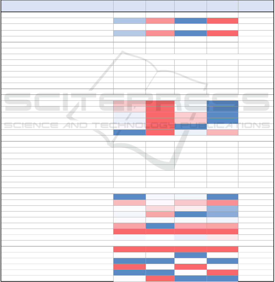
Figure 9: This shows the quarterly migration from all the techniques across all the markets.

4.3 Business Recommendations

The profiling helped in providing business

recommendations related to the following business

problems.

1. Identifying the key categories for the stores in

order to make a strategic decision. Category 4

is dominant in cluster 3 indicating the stores

belonging to cluster 3 should focus more on

category4.

2. For each cluster, an index can be created using

dimensions like average spend per transaction,

average units per transaction etc. These index

scores can then be leveraged to identify the

categories for each cluster which have the

maximum potential to grow.

3. Identifying the top performing stores. Cluster

3 has the maximum sales share but per store

sales is maximum for cluster 4 indicating that

cluster 4 stores on average performed better

than others.

4. Customer preferences are captured across

stores. For instance, cluster 2 has the

maximum number of Loyalty customers

followed by cluster 4. However, the Loyal

customer points redemption is the most in

cluster 4 which means promotions are most

effective for cluster 4 stores.

5. Understanding store firmographics to

optimize product portfolio. Cluster 1 has

mostly small size stores whereas cluster 3 has

medium type stores and cluster 2 / 4 are mostly

made up of large stores. This information

would help in space optimization planning for

each cluster type.

4.4 Scoring

The clustering techniques used above are

unsupervised learning algorithms, this essentially

means that there is no dependent variable in the

modelling exercise. In case, a new store is entering

a market then these algorithms cannot be applied to

classify the new store among one of the existing

clusters. To overcome this, machine learning

techniques such as Random Forest/Support Vector

Machines are applied. Here, the independent

variables are chosen out of the set of clustering

modelling variables and the dependent variable is

cluster mapping of each store. Hence, this is the

classic use case of multinomial classification. Once,

the prediction model is built, this model is further

used to score on the existing/new stores at a set

frequency (Quarterly/Semi-Annually/Annually).

Market Quarters Q2 '17 - Q3 '17 Q3 '17 - Q4 '17 Q4 '17 - Q1 '18 Q1 '18 - Q2 '18 Average

Hierarchical

11.8% 13.6% 11.0% 8.5%

11%

FCM

14.3% 15.8% 7.4% 11.0%

12%

GMM

12.2% 12.9% 7.8% 8.8%

10%

SOM

10.4% 10.0% 6.4% 4.2%

Hierarchical

7.8% 10.9% 7.8% 9.3%

FCM

3.9% 5.6% 7.4% 8.4%

GMM

2.8% 5.5% 6.8% 8.8%

SOM

4.2% 3.9% 4.6% 4.2%

Hierarchical

7.6% 7.2% 4.9% 4.9%

FCM

3.4% 5.1% 6.9% 6.8%

GMM

2.3% 3.2% 3.6% 4.0%

SOM

3.7% 3.4% 4.1% 3.7%

Hierarchical

2.1% 1.5% 1.1% 3.8%

FCM

3.5% 1.6% 1.1% 2.9%

GMM

2.6% 3.5% 4.5% 3.4%

SOM

4.2% 1.7% 1.7% 3.3%

DATA 2019 - 8th International Conference on Data Science, Technology and Applications

4.5 Migration

To check the robustness of the model, migration

across quarters is calculated. For this, store level data

is prepared for 5 quarters. Stores belonging to the

quarters are scored using the prediction model built at

the earlier stage. For example, each store of Q2 and

Q3 of 2017 are scored (allocated a cluster). Then

migration is calculated across quarters. Migration is

the number of stores which have changed cluster

across the two quarters divided by the total number of

common stores across the two quarters. As shown in

figure 9, in market 1, the migration from Q2’17 to

Q3’17 using Hierarchical clustering is 11.8%. This

mean for 11.8% of the stores the cluster allotment

changed when the quarter changed from Q2 to Q3.

Lower migration implies that the model is robust.

Hence, quarterly migration is considered as one of the

most important criteria for choosing the best

technique.

As shown in figure 9, SOM performed the best for

market 1 and market 2 with an average migration

across quarters of about 7.8% and 4.2% respectively.

GMM is the best technique for market 3 with the

average migration of 3.3%. Hierarchical clustering

performed the best for market 4 with the average

migration of 2.1%, however, the results from fuzzy

logic are close. Different techniques performed

differently in each market.

5 CONCLUSIONS

The paper considers four clustering techniques

namely: Hierarchal Clustering, Self Organizing

Maps (SOM), Gaussian Mixture Matrix (GMM) and

Fuzzy C-means(FCM). The techniques are applied to

the retail database to cluster the stores with similar

profile together. Each technique has a different

approach to clustering. The main parameter for the

retailer to measure the effectiveness of the cluster is

quarterly migration. It is noticed that no technique is

the best for all the markets. SOM performed better in

two markets, however, GMM and Hierarchical

outperformed the other techniques in one market

each. So, it is concluded that it is difficult to

generalize one technique to be the best suited for store

clustering exercise. The data and the features

determine which technique is to be applied. From this

exercise, it is recommended different clustering

techniques should be performed and one with the best

results should be finally selected.

ACKNOWLEDGEMENTS

The authors would like to thank three reviewers who

assisted in reviewing the content and improving the

quality of the paper.

REFERENCES

Bilgic E., Kantardzic M. and Cakir O. (2015). Retail Store

Segmentation for Target Marketing.

Spiller, P. and Lohse, G. (1997). A classification of internet

retail stores. International Journal of Electronic

Commerce, 2(2), pp.29-56.

Boone, D. and Roehm, M. (2002). Retail segmentation

using artificial neural networks. International Journal

of Research in Marketing. 19(3), pp287-301.

Hammouda, K. and Karray, F. (2002). A comparative study

of data clustering techniques. Tools of Intelligent

Systems Design.

Laverenko, V. (2014). EM algorithm: how it works.[

image]. Available at https://www.youtube.com/

watch?v=REypj2sy_5U&t=338s

Alogobean.com, (2017). Self Organizing Maps Tutorials.

[image] Available at: https://www.superdatascience.

com/blogs/the-ultimate-guide-to-self-organizing-

maps-soms

Superdatascience.com, (2018). The Ultimate Guide to Self

Organizing Maps. [image]. Available at: https://

algobeans.com/2017/11/02/self-organizing-map/

Chavent, M., Kuentz, V., Liquet, B., Saracco, J. (2011).

ClustofVar: An R package for clustering of variables.

Journal of Statistical Software, 55(2)

Watkins, M. (2014). The rise of modern convenience store

in Europe. Available at: https://www.nielsen.com/

eu/en/insights/reports/2014/the-rise-of-the-modern-

convenience-store-in-europe.html

Comparative Analysis of Store Clustering Techniques in the Retail Industry