
Tsallis Divergence of Order ½ in System Identification Related
Problems
Kirill Chernyshov
a
V. A. Trapeznikov Institute of Control Sciences, 65 Profsoyuznaya Street, Moscow, Russia
Keywords: Tsallis Divergence, System Identification, Mutual Information.
Abstract: The measure of divergence and the corresponding Hellinger-Tsallis mutual information have been introduced
within the information-theoretic approach to system identification based on Tsallis divergence and Hellinger
distance properties for a pair of probability distributions to be used in statistical linearization problems. The
introduced measure in this case is used ambivalently: as mutual information, a measure of random vector
dependence, — as a criterion of statistical linearization of multidimensional stochastic systems, and as a
measure of divergence of probability distributions — as an anisotropic norm of input process used to quantify
the correspondence between the observable data and the assumptions of the original problem statement as
such.
1 PRELIMINARIES
The measure of inequality between continuous
multiple probability distributions, such as
and
of a -dimensional random vector , are well
known as measures of divergence, including
Kullback-Leibler divergence,
(1)
is probably the most widely known and applied tool
in various problems related to stochastic system
analysis. In (1) and below,
⋅
is a mathematical
expectation with respect to probability distribution .
Meanwhile, there are broader approaches that
enable the characterization of inequalities between
two probability distributions, including Kullback-
Leibler divergence. In particular, this includes α order
Tsallis (2009) divergence of continuous
multidimensional probability distributions, e. g.
and
, which is defined as follows:
(2)
a
http://orcid.org/0000-0003-4637-6161
As is known, if parameter α tends to 1 then value
‖
in (2) tends to
‖
in (1), and,
therefore, Kullback-Leibler divergence may be
treated as Tsallis divergence of the order 1.
The expedience of considering Tsallis divergence
in construction of an anisotropic norm is due to the
fact that Kullback-Leibler divergence (1) is a marginal
case of Tsallis divergence of the order α with α tending
to 1. Specifically, Tsallis divergence
21
ppD
T
1,0
in (2) is a straightforward generalization
of Kullback-Leibler divergence in replacing the
logarithm with an appropriate exponential:
At the same time,
In turn, Figure 1 depicts the function
ℓ
behavior with certain α values compared with the
conventional logarithmic function.
,
)(
)(
ln
2
1
21
1
z
z
E
p
p
ppD
p
KL
.1,0,
)(
)(
1
1
1
1
2
1
21
1
z
z
E
p
p
ppD
p
T
.1,0,0,
1
1
)(
1
z
z
z
.0),ln()(lim
1
zzz
Chernyshov, K.
Tsallis Divergence of Order 1/2 in System Identification Related Problems.
DOI: 10.5220/0007919105230533
In Proceedings of the 16th International Conference on Informatics in Control, Automation and Robotics (ICINCO 2019), pages 523-533
ISBN: 978-989-758-380-3
Copyright
c
2019 by SCITEPRESS – Science and Technology Publications, Lda. All rights reserved
523
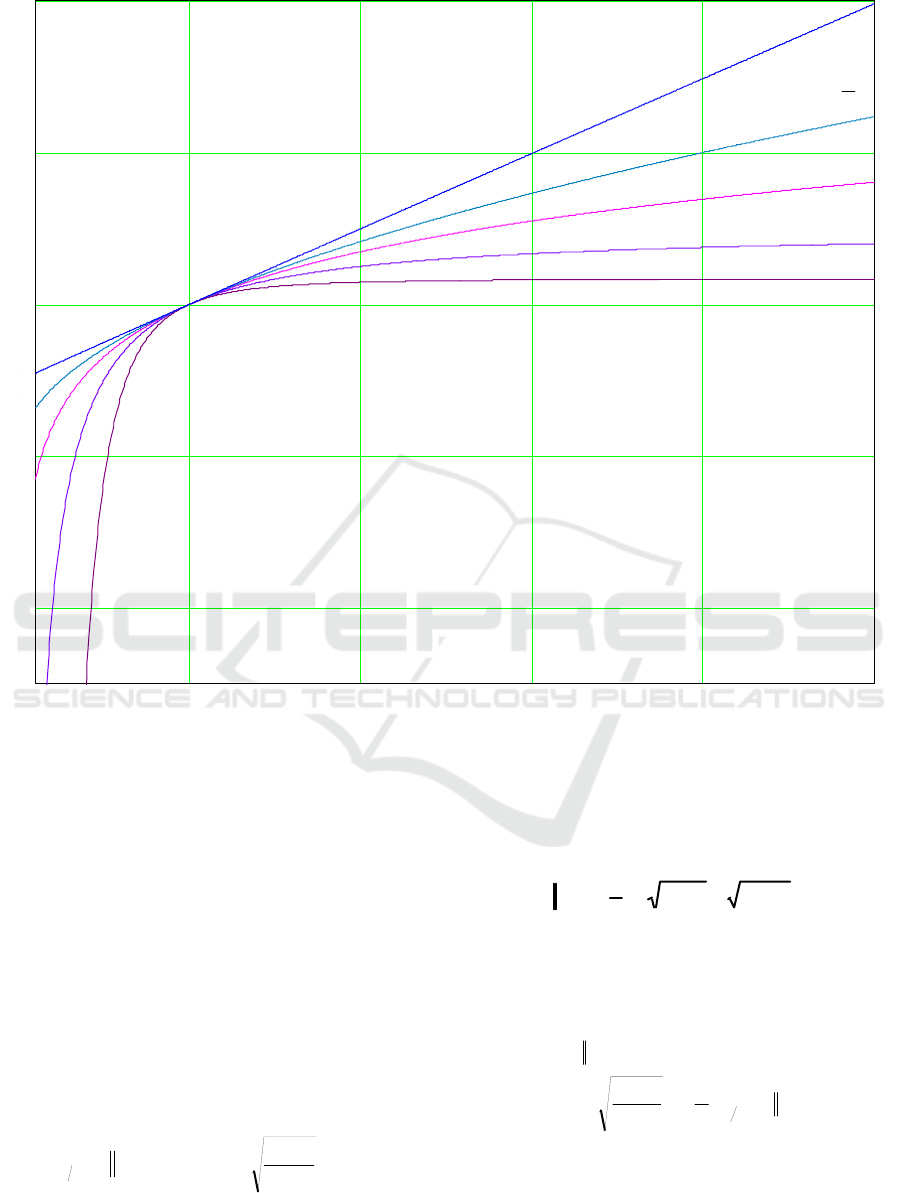
Figure 1: Plots of the logarithm and function ℓ
under certain values of parameter α.
From the computational point of view, especially
when calculations are based on sampled data, Tsallis
divergence is more useful compared to Kullback-
Leibler divergence as the latter includes an “integral
of logarithm”, which is generally recognized as more
complex for computational purposes compared to
Tsallis divergence, which includes no logarithm at all.
Meanwhile, the choice of a specific α order value is
important as the larger it is, the more complex the
computational process. On the other hand, there is
only one α value that renders Tsallis divergence
symmetrical relative to the probability distribution
densities being compared. This value is, obviously,
1
2
. Consequently, its analytic expression is as
follows:
(3)
On the other hand, it can be noted that
⁄
‖
is neither more nor less than double
Hellinger (1907) distance between probability
distributions defined as
(4)
where dim. Based on expressions (3) and (4),
Hellinger-Tsallis divergence is naturally defined as
follows:
(5)
Apart from the symmetry,
‖
is
characterized by the fact that its values fall within the
unit interval. This particular case of Tsallis
divergence will form the basis for further
1 2 3 4 5
4
2
0
2
4
.
)(
)(
12
1
2
21
21
1
z
z
E
p
p
ppD
p
T
,)()(
2
1
2
2121
2
R
dppppH zzz
.
2
1
)(
)(
1
21
21
1
2
21
1
ppD
p
p
ppD
T
p
HT
z
z
E
z
ln
2
2
1
4
1.0
ICINCO 2019 - 16th International Conference on Informatics in Control, Automation and Robotics
524

constructions within the framework of the approaches
applied in this article.
Measures of divergence may be treated as a
quality criterion in the context of various theoretical
and practical problems.
In particular, Hellinger-Tsallis divergence that is
defined by (5) results in an expression, which can be
referred as Hellinger-Tsallis
,
mutual
information for random vectors
and
of
dimensions
and
, respectively, where one
probability distribution density in
‖
, i. e.
,
, is a joint probability
distribution density of these random vectors, while
the other probability distribution density,
, is the product of marginal
probability distribution densities of
and
.
Similarly, the corresponding Hellinger-Tsallis
divergence
provides an
information theoretic quality criterion that may be
treated as a basis for creating an identification
criterion, which in turn defines the information
theoretic approach to system identification:
(6)
Handling the system identification problems is
always based on the use of various measures of
dependence of random values as is the case with the
input-output representation of the system in question
or with the approach to state-space description. In the
majority of cases, conventional linear
correlation/covariance measures of dependence are
used whose direct application results from the
identification problem statement itself if the case is
based on a conventional root mean square criterion.
The main advantage of these measures of dependence
is their usability: the feasibility of finding explicit
analytic expressions to define the necessary system
features and the relative simplicity of formulation of
their respective estimates, including those based on
the need to apply dependent observations.
Nonetheless, the chief deficiency of the linear
correlation-based measures of dependence is their
possible vanishing even in the presence of
deterministic dependence between random values
(Rajbman, 1981, Rényi, 1959).
More complex, nonlinear measures of
dependence are engaged to eliminate this deficiency
and to solve the stochastic system identification
problems. Among these measures, consistent
measures of dependence represent the main priority.
In accordance with A. N. Kolmogorov's
terminology, a measure of dependence for two
random values is treated as consistent where it
vanishes if and only if the above random values are
stochastically independent.
Statistical linearization of the system input-output
representation is actually related to nonlinear
identification problems whose solution is largely
defined by the characteristics of the input and output
processes dependence within the system in question.
On the other hand, the existing statistical linearization
approaches are based on the application of
conventional linear correlation, which, for reasons
stated above, may result in construction of models
with an output variable that is identically zero. In
particular, the likelihood of such result is shown using
an example in Section 5 in this article, which suggests
an approach focused on eliminating the identified
deficiencies and on applying consistent measures of
dependence within the framework of system
identification using linear representations of their
respective input/output models. The information
theoretic approach involves statement of the statistical
linearization problem for multidimensional discrete-
time systems.
2 PROBLEM STATEMENT
Let us assume that
is the n-dimensional output random system process
and
is the m-dimensional input random system process
within a multidimensional nonlinear dynamical
stochastic system. Within the framework of the above
process description, the processes and are
treated as stationary processes or mutually stationary
processes in a narrow sense. Then, the process
is white Gaussian noise with a covariance matrix
,
while the dependence of input and output system
processes is characterized (of which the researcher is,
naturally, not aware) by probability distribution
densities
.
),(
)()(
1
)()(),(
1,
21
21
212121
21
21
21
21
12
2121
2121
zz
zz
E
zzzzzz
ZZ
zz
zz
zzzz
zzzz
zz
p
pp
ddppp
IpppD
p
RR
HTHT
T
)(,),()(
1
tvtvtV
n
T
)(,),()(
1
sususU
m
Tsallis Divergence of Order 1/2 in System Identification Related Problems
525

(7)
For the sake of simplicity, but without loss of
generality, the vector-valued process components
and are treated with a zero mean and unit
variance,
(8)
where
⋅
is variance. Under the above terms,
(9)
A corresponding linear input/output system model
characterized by probability distribution densities (7)
is sought in the following form:
(10)
where
is the output process of the model,
, ∈
1,∞
, ,1,2,… are
matrix-valued (dimensions
) weight function
coefficients of a linearized model to be identified as
per the information theoretic criterion of statistical
linearization.
This criterion is a condition for coincidence of the
Hellinger-Tsallis mutual information (6) for the i
th
component,
, the system output process ,
and the j
th
component,
,the system input process
, which are characterized by the probability
distribution densities (7) and the Hellinger-Tsallis
mutual information (6) the for i
th
component,
,, the output process
,,, and the j
th
component,
, the input process of model
(10) for all
1,…,, 1,…,. From the
analytical point of view, this information-theoretic
criterion is expressed as follows:
(11)
As regards designations in criterion (11), it should
be noted that in the case of stationary and mutually
stationary, in the strict sense, random processes, e. g.
and
, Hellinger-Tsallis mutual
information is the corresponding function of time
:
where
,
;,
,
are mutual
and marginal probability distribution densities of
and
, , respectively.
By all means, from the viewpoint of a statistical
linearization problem, condition (11) must be
supplemented with a condition of coincidence of
mathematical expectations regarding the system and
model output processes,
(12)
It is evident that, within this problem description,
condition (12) is met automatically.
Moreover, in accordance with normalization
condition (8), model (10) output process components
are imposed upon the unit variance condition,
(13)
and, consequently, the sequences of matrix-valued
weight function coefficients of model (10) must meet
the following condition:
(14)
where
is the i
th
sequence of matrices ,1,2,… in
(10).
Relationship (14) is evidently defined by the
sequence as follows:
,2,1
,,1
,,,1
),;,(
,
mj
ni
uvp
ji
uv
,,,1,,,1
,1)()(
;0)()(
mjni
sutv
sutv
ii
ii
varvar
EE
.
1
1
)1(1
)1(
12
112
mmm
mm
m
U
cc
c
c
cc
C
,2,1,)()();(
ˆ
1
ttUWtV
W
T
WWW );(ˆ,),;(ˆ);(
ˆ
1
tvtvtV
n
.,2,1,,,1,,,1
,);(),,(
ˆ
);(),(
stmjni
sutvIsutvI
ji
HT
ji
HT
W
,
,
);,(
)()(
1
);(),(
21
21
21
21
21
21
st
zzp
zpzp
sztzI
zz
zz
p
HT
zz
E
.,,1,0);(
ˆ
)( nitvtv
ii
WEE
,,,1,1);(
ˆ
nitv
i
Wvar
,,,1,1)()(
1
niwCw
iUi
T
)(,),()(
1
imii
www
ICINCO 2019 - 16th International Conference on Informatics in Control, Automation and Robotics
526

based on the description of model (10) and
normalization conditions (8), (9). (13).
Therefore, expressions (11) and (12) are
information-theoretic criteria of statistical
linearization of the system that is represented by
probability distribution densities (7).
3 SOLUTION TECHNIQUE
As the first step, one can consider a sequence of
random values
being evidently Gaussian ones with the zero mean
and variance, due to (10), expressed as follows:
Then, within this set of notations,
1
-
dimensional vector
is Gaussian with corresponding covariance matrix
and the correlation for a bivariate Gaussian random
vector
;
can be written as
follows:
where
21
-dimensional matrix Ψ
is
expressed as follows:
and, as stated above,
,…,
are the
elements of the i
th
row of matrices from (10).
Hence, random vector
;
is
Gaussian with corresponding covariance matrix
expressed as follows:
(15)
Calculation of the right side of (15) results in
(16)
where
is the j
th
component of the column vector
.
Therefore, formula (6), above reasoning, and
formula (16) suggest that Hellinger-Tsallis mutual
information (6)
,,
; on input and
output model processes (10) (in other words, bivariate
Gaussian random vector
;
with covariance matrix defined by (11)) is expressed
as
which, in turn, based on condition (11), results in
)()(
)()()()(
)()()()(
)()();(
ˆ
1
1
1
1
T
T
TT
E
E
varWvar
iUi
qp
ii
ii
ii
wCw
qwqtUptUpw
wtUtUw
tUwtv
,2,1
,)()()()(
1
1
1
,
j
i
j
i
t
i
jtUjwjtUjw
.,2,1),()(1
)()(
)()(
1
1
1
,
T
T
T
var
iUi
j
iUi
j
iUi
t
i
wCw
jwCjw
jwCjw
T
)(,),(,),(
1
,
tutut
m
t
ii
),()(1)(
,
10
10
00)(
)1(1
)1(
12
112
),(
T
iUiij
mmm
mm
m
ij
t
wCw
cc
c
c
cc
C
i
),,()(
)(
);(
ˆ
t
tu
tv
iij
j
i
W
,
00100
)()()()(1
)(
)1(1
imjiiji
ij
wwww
).()()(
),(ˆ
T
ijtijuv
iji
CC
,
1)(
)(1
)(
ˆ
ij
ij
uv
ji
C
,,2,1,
)(det3
)(det
21
);(),,(
ˆ
ˆ
4
ˆ
st
C
C
sutvI
ji
ji
uv
uv
ji
HT
W
Tsallis Divergence of Order 1/2 in System Identification Related Problems
527
(17)
Expression (17), in turn, directly results in
(18)
Then, based on condition (11), the required
expressions for rows
of the matrix-valued
weight function coefficients
,1,2,… of
model (10) appear as follows:
(19)
where
(20)
In formulas (19) and (20)
is a regression
of
on
; sign
1 as 0,
sign
1 as 0 is a corresponding regression
function sign that represents “relative orientation” of
input and output process components, while value
,
; in (19), (20) is always non-
negative.
Moreover, the measure of dependence
,
; defined by expressions (6) and
(18) meets all Rényi (1959) axioms for measures of
random values dependence. Meanwhile, the
calculations here are much simpler than in the case of
the maximum correlation coefficient (Rényi (1959,
Sarmanov, 1963a,b).
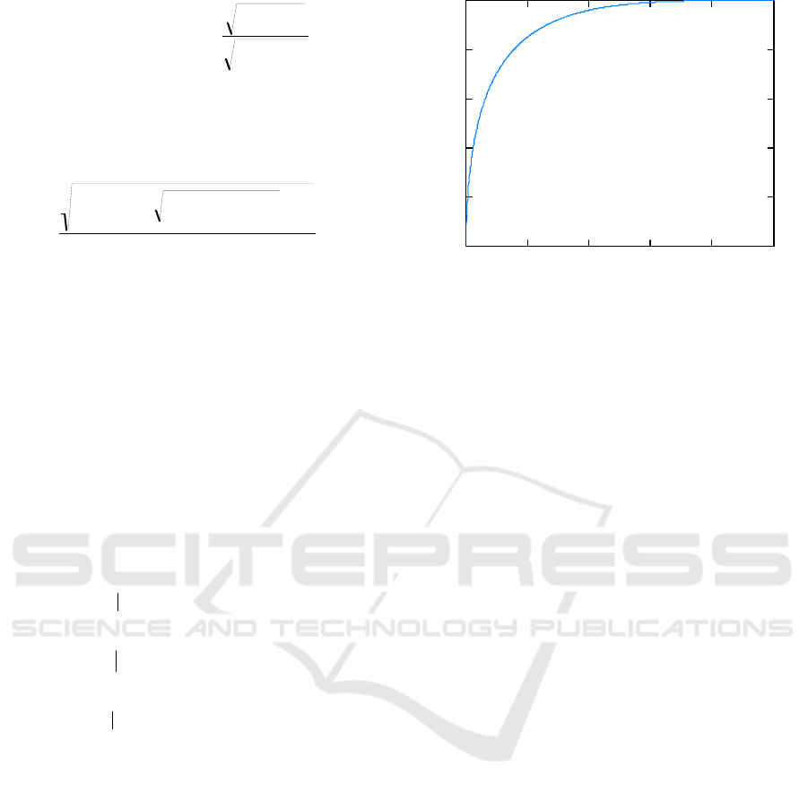
The behavior of measure of dependence (18) as a
function of
,
; is shown in Figure 2.
Figure 2: Behavior of measure of dependence
,
; (18) as a function of
,
;.
Therefore, vanishing of the weight function
coefficients of linearized model (10) within a
nonlinear system characterized by probability
distribution densities (7) is equivalent to vanishing of
Hellinger-Tsallis mutual information (6) on input and
output processes within the system in question. The
latter, in turn, is possible if and only if these processes
are stochastically independent. The direct
consequence of the above is that vanishing of all
weight function coefficients of linearized model (10)
indicates that the original nonlinear system is
unidentifiable. Meanwhile, as stated above, there are
examples of traditional measures of dependence
vanishing if there is stochastic dependence between
the system variables.
4 ZERO CORRELATION OF
INPUT AND OUTPUT
VARIABLES: EXAMPLE
There are multiple examples where the use of
conventional correlation methods within the
framework of the models obtained fails to provide
satisfactory results. Among such systems, it is
possible to distinguish those where input and output
processes dependence is characterized by probability
distribution densities that belong to O. V. Sarmanov
distribution class (Sarmanov, 1967, Kotz et al., 2000)
and expressed as
(21a)
with marginal probability distribution densities
and
,
,2,1
,
)(4
)(1
21);(),(
2
4
2
st
sutvI
ij
ij
ji
HT
.,2,1
,1);(),()(
,
)(
21)(31)(
2
);(),(
2
22
st
sutvI
sutv
ji
HT
ij
ij
ijij
ji
HT
,,2,1
,);(),()(
1
st
sUtvCw
i
HT
Ui
Ι
T
.,2,1
,
);(),()(sign
);(),()(sign
);(),()(sign
);(),(
1
1
st
sutv
sutv
sutv
sUtv
mi
HT
uv
ji
HT
uv
i
HT
uv
i
HT
mi
ji
i
m
m
m
Ι
0 0.2 0.4 0.6 0.8
0
0.2
0.4
0.6
0.8
,)()(1)()(),(
21;
vuvpupuvp
vuvu
);(),( swty
ji
HT
));(),((
sxtyI
HT
ICINCO 2019 - 16th International Conference on Informatics in Control, Automation and Robotics
528
(21b)
where parameter λ meets the condition:
(21c)
Correlation coefficient and correlation ratio for
probability distribution densities (21) are equal to
zero. Let’s consider the following probability
distribution density that belongs to O. V. Sarmanov
distribution class:
(22)
Its marginal probability distribution densities are
Laplacian ones.
Meanwhile, the maximum correlation coefficient
for probability distribution density (22), hereinafter
designated as
, is expressed as follows:
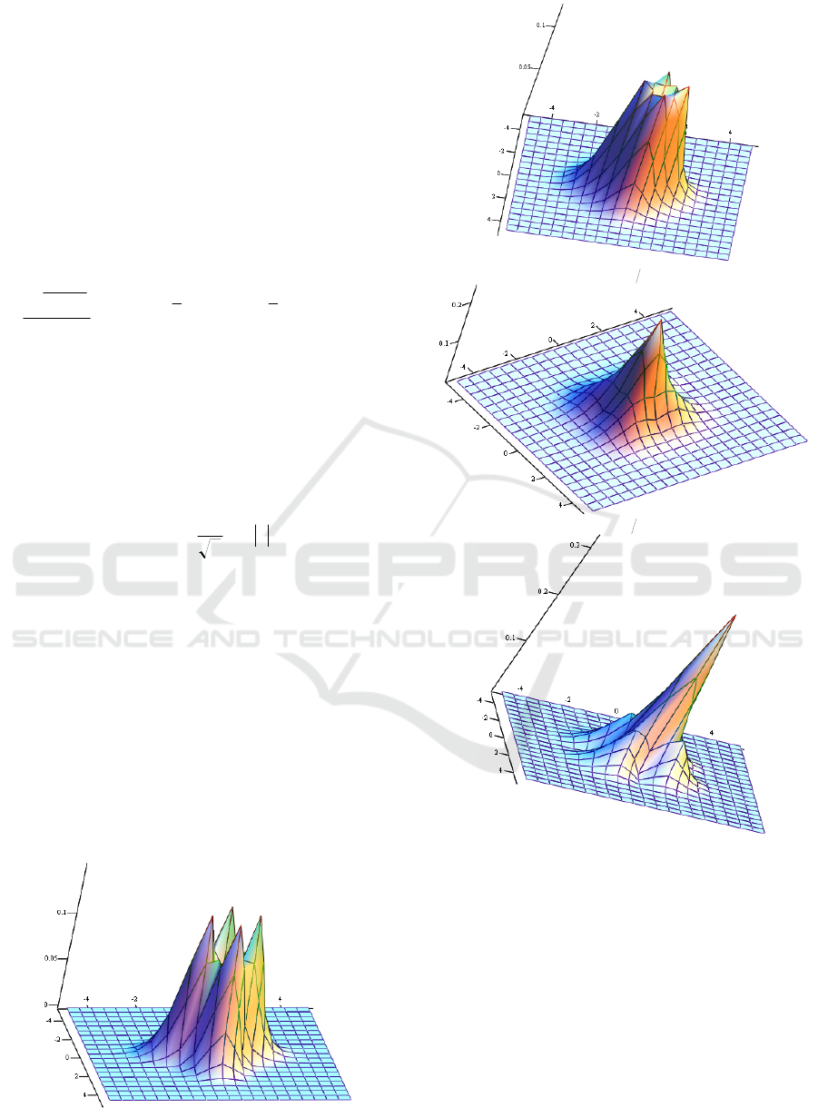
The value of parameter λ has a significant impact
on the form of probability distribution density (22).
Figure 3 depicts probability distribution density (22)
for certain values of parameter λ.
Let us assume that in (7), the joint probability
distribution density is p_λ (v,u) of (22). Then, the
Hellinger-Tsallis mutual information for the
probability density function p_λ (v,u) may be a
corresponding function of parameter λ to be
designated as I^HT (λ). Consequently, measure of
dependence (18) for probability distribution density
p_λ (v,u) (22) will be designated as ι^HT (λ),
respectively.
Figure 3: Shape of probability distribution density (22) for
certain values of parameter λ.
Figure 4 depicts the behavior of
as a
function of parameter λ of probability distribution
density (22) compared with the corresponding values
of the maximum correlation coefficient
.
clearly shows the dependence between
random values, which basically matches (formally,
even to a greater extent) the maximum correlation.
For example, if stochastic dependence (7) between
the components of the output process,
, and the
input process,
, of a nonlinear stochastic system
,0)()(,0)()(
21
dvvvpduuup
vu
.0)()(1
21
vu
.11
,12121
2
),(
22
22
2
3
2
3
2
uv
uv
ee
e
uvp
.1
7
4
)(
vu
S
1
21
21
1
Tsallis Divergence of Order 1/2 in System Identification Related Problems
529
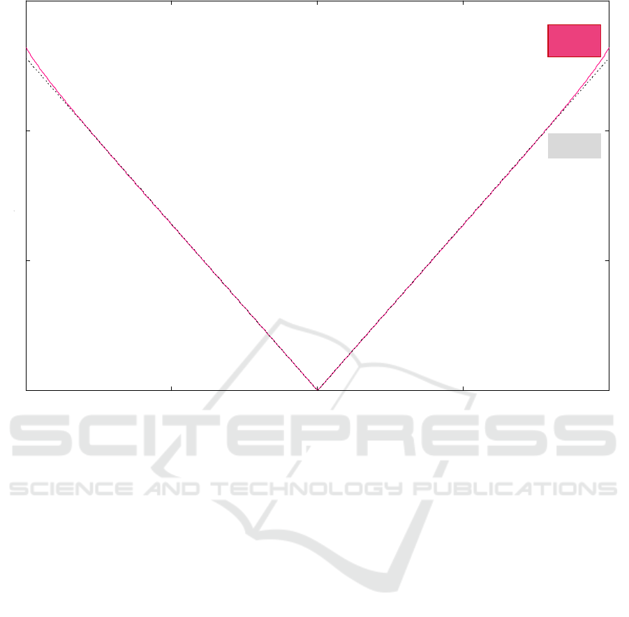
Figure 4: Behavior of
(unbroken line) as a function of parameter λ of probability distribution density (22) compared
with the corresponding values of the maximum correlation coefficient
(broken line).
is defined by a probability distribution density (of
which the researcher is, naturally, not aware) of type
(21) with parameter
, , then the
use of conventional correlation methods within the
framework of model (10) being constructed will
result in a representation of the output model process
as a null equation, which is excluded within the
framework of the proposed information-theoretic
approach.
5 HELLINGER-TSALLIS
MUTUAL INFORMATION
ESTIMATION
As far as the problem of obtaining estimates for
weight function coefficients (19) of linearized model
(10) by using the data from sample observation of the
input and output process values in a system
characterized by joint probability distribution
densities (7) is concerned, a need arises for a
corresponding estimation of the Hellinger-Tsallis
mutual information (6); this type of problems allows
for a direct application of the Sklar (1959) theorem
regarding the representation of joint probability
distribution densities through their copula functions.
In particular, for joint probability distribution density
, of random values V and U with
corresponding marginal probability distribution
densities
,
, the following expansion is
valid:
(23)
where
are the functions of marginal probability distribution
densities of random values V and U, and
,
is the copula density function (for
copulas, refer to book of Nelsen (2006) and other
sources).
In accordance with representation (23), Hellinger-
Tsallis mutual information (6) is expressed as
follows:
1 0.5 0 0.5 1
0
0.2
0.4
),()()(),(),( upvpuPvPcuvp
uvuvvu
u
uu
v
vv
dxxpuPdyypvP )()(,)()(
HT
)(
vu
S
ICINCO 2019 - 16th International Conference on Informatics in Control, Automation and Robotics
530

(24)
Representation (24) enables the application of the
mutual information estimation (according to Shannon
type) (Zeng and Durrani, 2011). Meanwhile, an
example of Hellinger-Tsallis mutual information
shown in formula (24) within the context under
consideration is even more simple since the copula
density function based on representation (23) in the
case of Shannon mutual information still includes the
logarithm of the copula density function:
Meanwhile, complications inherent in the division
operations may be avoided through the use of methods
for copula density function estimation instead of
probability density function estimation.
6 ANISOTROPIC NORM BASED
ON THE HELLINGER-TSALLIS
DIVERGENCE
The approach in question is based on the assumption
that the m-dimensional process of the input system
is 1) white noise, and 2) is Gaussian. These
assumptions may be checked by using an anisotropic
norm as a quantitative measure. Anisotropic norm for
a random vector was shown in (Vladimirov et al.,
1995, 1999) based on the Kullback-Leibler
divergence, which automatically results in its
nonsymmetry.
Namely, the definition of the anisotropic norm for
random m-dimensional vector
U with covariance
matrix C and probability distribution density
)(Up
U
, which is based on Kullback-Leibler divergence, and
is expressed as follows:
,
)(
)(
ln)(min
0
m
R
U
U
a
dU
UG
Up
UpU
where
)(UG
is the probability distribution density of
an n-dimensional Gaussian random vector with a so-
called a scalar covariance matrix
m
I
, where
m
I is
a unit
mm
-matrix:
.
2
1
)(
2
2
U
m
eUG
The key feature and benefit of using Kullback-
Leibler divergence to define the anisotropic norm
a
U
in that form is the possibility to solve explicitly
the optimization problem that is behind definition of
the anisotropic norm
a
U
, since such a solution is
determined by equation
,0
)(
)(
ln)(
m
R
U
U
dU
UG
Up
Up
d
d
where optimum value
is expressed as
.
2
m
UE
Under this value of
, the above definition of the
anisotropic norm
a
U
immediately takes on its
closed form
,2ln
2
2
U
UE
C
a
S
m
e
m
U
where
)(U
C
S is Shannon entropy of m-dimensional
random vector
U with the covariance matrix C:
.)(ln)()(
m
R
UUC
dUUpUpS U
It should be noted that this simple solution is
achieved solely through introducing logarithm of
exponent in definition of the anisotropic norm
a
U
.
Again, definition of Vladimirov et al. (1995,
1999) is based on a comparison between this
Gaussian probability distribution density of random
vectors with a scalar covariance matrix. The latter
may be treated as an excessive limitation. In turn,
Chernyshov (2018) has proposed an approach to
define anisotropic norms, which would be both
symmetrical and vanishing for any Gaussian vector
with a particular focus on Hellinger-Tsallis
divergence as naturally assuming unit interval values
by default. Therefore, such anisotropic norm of an m-
dimensional random vector
with a
probability distribution density
with
covariance matrix
is expressed as
.)()();(),(1
)()();(),(1
);,(
)()(
1);(),(
1
0
1
0
udPvdPuPvPc
dvduupvpuPvPc
uvp
upvp
sutvI
uvuv
uvuv
vu
uv
ji
HT
E
.);(),(ln);(),(
uPvPcuPvPc
uvuv
Tsallis Divergence of Order 1/2 in System Identification Related Problems
531

(25)
where
is the probability distribution density for
Gaussian m-dimensional vector with the same
covariance matrix
. It is evident that
‖
‖
0 for the Gaussian property of .
Then, in order to characterize Gaussian and white
noise properties (mutual independence) typical of an
(infinite) sequence of signals, the mean anisotropic
norm (Vladimirov et al., 2006) is defined by a
corresponding anisotropic norm for a single random
vector. In other words, assume
(26)
with a sequence of m-dimensional random vectors,
and
(27)
Then the mean anisotropic norm for sequence (26)
is defined by Vladimirov et al. (2006) as
(28)
with
‖
‖
being understood in terms of definition
of Vladimirov et al. (1995, 1999).
In turn, as per definition (25), the mean
anisotropic norm for vector sequence (26) is naturally
defined as
(29)
where
(30)
In turn,
in (30) designates the probability
distribution density for
⋅
-dimensional random
vector (27), and
is a
⋅
-dimensional
Gaussian random vector with covariance matrix
(31)
where, as above,
is covariance matrix ,
1,2,…
in (26).
Therefore, we may arrive at the conclusion that if
the input process
, 1,2,… meets the
conditions of statistical linearization problem
statement, the maximum possible value
of the mean
anisotropic norm for the input process
,
1,2,…
, defined in (29)-(31), must be set. In other
words, if
(32)
then the input process
1,2,… meets the
conditions of the original problem statement,
otherwise, the conditions are not met. Meanwhile, if
a type (32) condition is introduced, it is essential that
the anisotropic norm is defined by Hellinger-Tsallis
divergence and its values fall within the unit interval.
This approach is by all means purely theoretic as
it suggests that the corresponding probability
distribution density
is known for any value of N, which is usually not the
case, and the value of
‖
‖
is to be found by sample
observation of the input system
process. In
practice, cases when such direct estimation is possible
are rare due to an enormous volume of the sampled
data to be handled given that N is relatively large.
On the other hand, within the framework of
definitions (29)-(31), condition (32) is essentially a
test for both white noise (mutual independence) and
Gaussian properties. Thus, condition (32) will be met
if for any two input vectors in the system, e. g. for
and , in particular case (30), i. e. for type
|
2
|
, the following condition is met:
(33)
where
(34)
Condition (33) is, naturally, more strict than (32);
however, it is much easier to check. Therefore,
Parzen-Rosenblatt kernel density estimates and
respective methods based on approach (Mokkadem,
1989) to estimate Shannon mutual information are
used to build estimates of
|
|
in (33) via sample
observation of
2-dimensional random vector (34).
Meanwhile, regarding Hellinger-Tsallis divergence
the estimation procedure becomes considerably
simpler than that of Shannon mutual information case
namely due to the absence of the necessity to make the
limit transfer concerned with presence of the integral
of logarithm in Shannon mutual information, with
,)(
U
C
U
HT
HT
a
GpDsU
,2,1),( ssU
.)(,),1(
T
TT
U NUU
N
,lim
N
a
N
N
a
U
U
,lim
HT
a
N
N
HT
a
UU
.
G
N
N
CHT
HT
a
N
GpD
U
U
U
,
Ummmm
mm
Umm
mmmmU
G
N
C
C
C
C
00
0
0
00
U
,
HT
a
U
)(,),1( NUUpp
NN
TT
UU
,
2
2
2
G
CHT
HT
a
GpD
U
U
U
.)(),(
2
T
TT
U jUiU
ICINCO 2019 - 16th International Conference on Informatics in Control, Automation and Robotics
532

being absent the logarithm in Hellinger-Tsallis
divergence.
7 CONCLUSIONS
This paper treats the problem of statistical
linearization for nonlinear multidimensional
dynamical stochastic systems described by input-
output representation with an input process of a
Gaussian white noise type as a construction of
equivalent linear input-output model as per the
information-theoretic criterion based on Hellinger-
Tsallis mutual information (6). The latter resulted in
equations enabling the determination of the linearized
model weight matrix elements, which define them as
a function of Hellinger-Tsallis mutual information,
while vanishing of mutual information is equivalent to
vanishing of the respective weight matrix elements.
Meanwhile, this is equivalent to independence of the
respective components of the input and output
processes of the initial system under study, which, in
turn, is indicative of the identifiability of such a
system.
REFERENCES
Chernyshov, K. R., 2018. “The Anisotropic Norm of
Signals: Towards Possible Definitions”, IFAC-
PapersOnLine , vol. 51, no. 32, pp. 169-174.
Hellinger, E. D., 1907. “Die Orthogonalinvarianten
quadratischer Formen von unendlich vielen Variablen”,
Thesis of the university of Göttingen, 84 p.
Kotz, S., Balakrishnan, N., and N. L. Johnson, 2000.
Continuous Multivariate Distributions. Volume 1.
Models and Applications / Second Edition, Wiley, New
York, 752 p.
Mokkadem, A., 1989. “Estimation of the entropy and
information of absolutely continuous random
variables”, IEEE Transactions on Information Theory,
vol. IT-35, pp. 193-196.
Nelsen, R. G., 2006. An Introduction to Copulas / Second
Edition, Springer Science+Business Media, New York,
2006, 274 p.
Rajbman, N. S., 1981. “Extensions to nonlinear and
minimax approaches”, Trends and Progress in System
Identification, ed. P. Eykhoff, Pergamon Press, Oxford,
pp. 185-237.
Rényi, A. 1959. “On measures of dependence”, Acta Math.
Hung., vol. 10, no. 3-4, pp. 441-451.
Sarmanov, O. V., 1963a. “The maximum correlation
coefficient (nonsymmetric case)”, Sel. Trans. Math.
Statist. Probability, vol. 4, pp. 207-210.
Sarmanov, O. V., 1963b. “Maximum correlation coefficient
(symmetric case)”, Select. Transl. Math. Stat. Probab.
vol. 4, pp. 271-275.
Sarmanov, O. V., 1967. “Remarks on uncorrelated
Gaussian dependent random variables”, Theory
Probab. Appl., vol. 12, no. 1, pp. 124-126.
Sklar, A., 1959. “Fonctions de répartiticion à n dimensions
et leurs marges”, Publ. Inst. Statist. Univ. Paris 8, pp.
229-231.
Tsallis, C., 2009. Introduction to Nonextensive Statistical
Mechanics. Approaching a Complex World, Springer
Science+Business Media, New York, 388 p.
Vladimirov, I. G., Diamond, P., and P. Kloeden, 2006.
“Anisotropy-based robust performance analysis of
finite horizon linear discrete time varying systems”,
Automation and Remote Control, vol. 67, no. 8, pp.
1265-1282.
Vladimirov, I. G., Kurdjukov, A. P., and A. V. Semyonov,
1995. “Anisotropy of Signals and the Entropy of Linear
Stationary Systems”, Doklady Math., vol. 51, pp. 388-
390.
Vladimirov, I. G., Kurdjukov, A. P., and A. V. Semyonov,
1999. “Asymptotics of the anisotropic norm of linear
discrete-time-invariant systems”, Automation and
Remote Control, vol. 60, no. 3, pp. 359-366.
Zeng, X. and T. S. Durrani, 2011. “Estimation of mutual
information using copula density function”, Electronics
Letters, vol. 47, no. 8, pp. 493-494.
Tsallis Divergence of Order 1/2 in System Identification Related Problems
533
