State Observers for Mechatronics Systems with Rigid and Flexible
Drive Dynamics
Alexandra-Iulia Szedlak-Stinean, Radu-Emil Precup and Radu-Codrut David
Department of Automation and Applied Informatics, Politehnica University of Timisoara,
Bd. V. Parvan 2, 300223, Timisoara, Romania
Keywords: State Observers, Electromechanical Plant, Experimental Results, Rigid Drive Dynamics, Flexible Drive
Dynamics, Adjustable Moment of Inertia.
Abstract: The mechatronics systems with rigid and flexible drive dynamics are nonlinear and complex processes. This
paper proposes a controller with a novel structure, which is composed of three subsystems: a subsystem that
provides the desired output and from the reference input a feed-forward signal, an observer and a feedback
derived from the estimated states. This structure has the advantage that the response to reference signals can
be decoupled from the response to disturbances. This paper also proposes observers based on predictive
feedback, characterized by fast convergence and small sensitivity of the estimation to parameter variations.
Design approaches for the controller and state observers are offered. The experimental setup considered in this
paper, namely the Model 220 Industrial Plant Emulator (MIPE220), illustrates how the use of several control
structures can be made accessible, easily understandable and increasingly attractive. The proposed design
approaches are tested and validated in terms of conducting real-time experiments in terms of two experimental
scenarios – step and staircase reference inputs – obtained for three specific values of the moment of inertia of
the load disk.
1 INTRODUCTION
Mechatronics systems have experienced a fast and
complex multidisciplinary development as a result of
advances in various fields of applications such as
(Isermann, 2005; Bishop, 2007; Gutiérrez-Carvajal et
al., 2016): expert systems, automotive engineering,
robotics and automation, structural dynamic systems,
machine vision, control systems, servo mechanics,
numerical computing systems based on
microelectronics with a high degree of integration,
consumer products, medical imaging systems, mobile
apps, computer-aided and integrated manufacturing
systems, transportation and vehicular systems, etc.
The development of linear and nonlinear observers
has led over the years to a novel stage of engineering
design. Luenberger was the first to introduce and
solve the problem of designing observers for linear
control systems (Luenberger, 1966). One of the
central problems in control systems literature,
designing observers for nonlinear control systems,
was proposed in (Thau, 1973). In the hypothesis of
linearity of the process model, the basic structure of
the observer is always the same, but its realization
will depend on the chosen context: continuous or
discreet, deterministic or stochastic. An observer is
very useful for implementing feedback stabilization
or feedback regulation due to the fact that it is
essentially an estimator for the state of the system,
and some representative papers on this subject are
(Brown and Hwang, 1996; Aghannan and Rouchon,
2003). The development of suitable algorithms to
perform the estimation has been the focus of many
researchers’ attention and for this purpose, in order to
estimate state variables from the available
measurements, several techniques have been
developed and introduced (Brown and Hwang, 1996;
Aghannan and Rouchon, 2003; Marx et al., 2007;
Lendek et al., 2008; Spurgeon, 2008; Magnis and
Petit, 2016). In this context, the paper proposes a
controller that can be considered as composed of
three subsystems: a subsystem that provides the
desired output and from the reference value a feed-
forward signal, an observer and a feedback derived
from the estimated states. The interesting structure of
the controller allows it to be applied for a wide range
of design methods. The controller structure and the
forms of the equations are exactly the same for
Szedlak-Stinean, A., Precup, R. and David, R.
State Observers for Mechatronics Systems with Rigid and Flexible Drive Dynamics.
DOI: 10.5220/0007921203870394
In Proceedings of the 16th International Conference on Informatics in Control, Automation and Robotics (ICINCO 2019), pages 387-394
ISBN: 978-989-758-380-3
Copyright
c
 2019 by SCITEPRESS – Science and Technology Publications, Lda. All rights reserved
387

systems with one input and one output as well as for
systems with multiple inputs and outputs. The same
controller structure can be obtained by employing
many other design techniques. The defining feature of
a state feedback controller and an observer have is the
complexity of the controlled system that determines
controller’s complexity. As such a system model is
actually contained by the controller. Thereby the
internal model principle that prescribes that an internal
model of the controlled system should be contained in
the controller is in this paper exemplified.
This paper offers the next five contributions over
the literature: 1. development of the dynamic
equations used in the process mathematical models
(MMs) of MIPE220 with rigid and flexible drive
dynamics and the interpretation of these MMs as
benchmark type models, 2. design approaches and
implementation of state observers in three case
studies dedicated to the position control of MIPE220
with rigid and flexible drive dynamics, 3.
development of Matlab/Simulink programs to test the
new control system structures, 4. experimental
validation of proposed techniques, and 5. a
comparative analysis of all design approaches for two
experimental scenarios to highlight how the specified
control system performance is achieved.
The paper discusses the following topics: the
dynamic equations that characterize the
electromechanical subsystem with rigid and flexible
drive dynamics are pointed out in Section 2.
Numerical values related to the MIPE220 are also
given in Section 2. The proposed design approaches
for the position control of a mechatronics system are
discussed in Section 3. Section 4 presents
experimental results concerning the implementation
of the developed design approaches and also a
comparative analysis of all control solutions. The
main conclusions are highlighted in Section 5.
2 DYNAMIC EQUATIONS AND
NUMERICAL VALUES FOR
THE ELECTROMECHANICAL
SUBSYSTEM MIPE220
The structure of the mechatronics application that
represents the controlled process (MIPE220) is
presented in Figure 1. The dynamic equations that
describe the mechatronics system in case of rigid (a)
and flexible (b) drive dynamics, considering θ
1
as the
process output are:
Figure 1: MIPE220 laboratory equipment.
.0)()(
,)()()
,)()
1
1
2
.
1
1
12
.
2122
..
2
2
1
1
2
.
2
1
12
.
1
2
121
..
1
.
1
2
21
..
1






gkgcccJ
TggkgcgccJb
TgccJa
l
Ddr
Ddr
(1)
with J
dr
, J
d
, J
l
, J
p
, g and g
’
expressed as
.12/',/6
,,
,
2
2
'
pdplpd
wlddldlbacklashpldpdrp
wdrddrdlpddr
ng nng
JJJJJJJ
,JJJ gJgJJJ





(2)
where J
dr
– total inertia reflected to the drive disk, Jp,
Jd, Jl, – pulley, drive disk and load disk inertia, c1, c2
– the drive and load friction, g, g’ – drive gear and
partial gear system ratio, θ1, θ2, θp – drive disk, load
disk and idler pulleys positions where θ
1=gθ2 or
θ1=g’θp.
2.1 Rigid Drive Dynamics
The first principle equations that describe the system
in case of rigid drive dynamics are (ECP, 2010;
Szedlak-Stinean et al., 2016):
















.
,
''
)(
,
1
2222
2
2
21
2
21
xy
gJgJJ
T
gJgJJ
xgcc
x
xx
dpd
D
lpd


(3)
The state-space MM (SS-MM) of MIPE220 with
rigid drive dynamics is
.]xx][01[
,
gJg'JJ
1
0
x
x
gJg'JJ
)gc(c-
0
10
21
2
l
2-
pd
2
1
2
l
2-
pd
2-
21
2
1
T
D
y
T
x
x




































(4)
where T
D is the drive torque (T
D
=u), x=[x
1
x
2
]
T
= [θ
1
dθ
1
/dt]
T
is the state vector (T indicates matrix
transposition) and y is the output. Considering zero
initial conditions, the application of the Laplace
transform to (1a)) leads to the following transfer
function (t.f.):
ICINCO 2019 - 16th International Conference on Informatics in Control, Automation and Robotics
388

,
)]gJg'JJ/()([
)gJg'JJ/(1
)(
)(
2
l
2-
pd
2
21
2
l
-2
pd
1





gccsssT
s
D
(5)
Using (4) and (5) the matrices A, B and C related to
the SS-MM and the t.f.s for three significant values of
the moment of inertia of the load disk are given in
Table 1 (ECP, 2010; Szedlak-Stinean et al., 2016).
Table 1: SS-MM matrices and transfer functions
expressions of MIPE220 with rigid drive dynamics.
Inertia Matrices A, B and C
Process
transfer
function
)(/)(
1
sTs
D

1
l
J

01,
7036
0
,
8.630
10















 CBA
)63.8(
7036
ss
2
l
J
 01,
4362
0
,
5.350
10















 CBA
)35.5(
4362
ss
3
l
J
 01,
2741
0
,
37.30
10















 CBA
)37.3(
2741
ss
2.2 Flexible Drive Dynamics
The first principle equations that describe the system
in case of flexible drive dynamics are (ECP, 2010):



























.
,
)(
)(
)()(
,
,
)()(
,
1
.
412232
1
121
1
4
43
1
12
1
2
2
1211
2
2
21
xy
J
xcc
J
xk
J
xgc
J
xkg
x
xx
J
gc
J
kg
J
xgcc
J
xkg
x
xx
llll
drdrdrdr




(6)
The SS-MM of MIPE220 with flexible drive
dynamics is
.]xxxx][0001[
,T
0
0
gJg'JJ
1
0
x
x
)(
1000
)()(
0010
4321
D
2
l
2-
pd
4
3
2
1
122
1
12
1
1
12
12
121
2
4
3
2
1
T
llll
drdrdrdr
y
x
x
J
cc
J
k
J
gc
J
kg
J
gc
J
kg
J
gcc
J
kg
x
x
x
x




































































(7)
where T
D is the drive torque (T
D
=u, u is the input),
x=[x
1
x
2
x
3
x
4
]
T
=[θ
1
dθ
1
/dt θ
2
dθ
2
/dt]
T
is the state vector
and y is the output. The following t.f. is attached to
(7):
,
)(
)(
)(
1
2
2
3
3
4
4
122
2
1
sdsdsdsd
ksccsJ
sT
s
l
D




(8)
where d
4
=J
dr
J
l
, d
3
=J
dr
(c
2
+c
12
)+J
l
(c
1
+c
12
/g
2
),
d
2
=J
dr
k+J
l
k/g
2
+c
1
c
2
+c
1
c
12
+c
12
c
2
/g
2
, d
1
=c
1
k+c
2
k/g
2
.
Using (7) and (8) the matrices A, B and C and the
t.f.s. related to MIPE220 with flexible drive dynamics
for three values of the moment of inertia of the load
disk are given in Table 2 (ECP, 2010; Szedlak-
Stinean et al., 2017).
2.3 MIPE220 Parameters Values
For the development of the proposed design
approaches, the parameter values for the
electromechanical subsystem, as presented in the
manual (ECP, 2010), are shown in Table 3.
Due to the fact that the employed laboratory
equipment does not permit a continuous variation of
the moment of inertia, the suggested control solutions
which will be tested and validated through
experiments are designed for three specific load disk
inertia values, J
li
,
}3,2,1{

i
(ECP, 2010; Szedlak-
Stinean et al., 2016; Szedlak-Stinean et al., 2017): the
low value J
l1
=0.0065kgm
2
(load disk without any
weights on it), the middle value J
l2
=0.01474kgm
2
(load disk has four 0.2 kg weights on it) and the high
value J
l3
=0.0271kgm
2
(load disk has four 0.5 kg
weights on it).
3 STATE FEEDBACK AND
OBSERVER-BASED
CONTROLLER DESIGN
In cases where the process states are not accessible for
measurements or are only partially accessible for
measurements and if the process is observable, then it
is possible to estimate its states. For this purpose, state
estimators or state observers are utilized. The
observability test of the linearized SS-MMs (4) and (7)
can be done using the matrix
....][
TTTTTT
o
CCCACC
432
AAAQ 
(9)
The numerical values specific to the analyzed
mechatronics application given in Tables 1 and 2 are
used in the computation of the rank of Q
o
.
The starting point in order to specify the relations
that describe the functioning of a state observer, is the
SS-MM corresponding to the process, assumed
known, with the form
.
,
xC
BxAx



y
u

(10)
State Observers for Mechatronics Systems with Rigid and Flexible Drive Dynamics
389

Table 2: SS-MM matrices and transfer functions expressions for MIPE220 with flexible drive dynamics.
Inertia Matrices A, B and C
Process transfer function
)(/)(
1
sTs
D

1
l
J
]0001[,
0
0
13850
0
,
307.10
1
13.10
0
1300
0
5036
0
654.0
0
068.12
1
325
0
1259
0




























 CBA
)220782.267737.22(
)1300307.10(13850
23
2


ssss
ss
2
l
J

0001,
0
0
13850
0
,
59.4
1
13.10
0
579
0
5036
0
3.0
0
068.12
1
145
0
1259
0




























 CBA
)4.98277.189365.16(
)57959.4(13850
23
2


ssss
ss
3
l
J
]0001[,
0
0
13850
0
,
47.2
1
13.10
0
312
0
5036
0
157.0
0
068.12
1
9.77
0
1259
0




























 CBA
)4.52904.159953.14(
)31247.2(13850
23
2


ssss
ss
Table 3: MIPE220 parameter values.
Electromechanical subsystem MIPE220 parameter values
Parameters Values Remarks
J
ddr
0.00040 [kgm
2
]
J
dld
0.0065 [kgm
2
]
J
b
acklash
0.000031 [kgm
2
]
J
wdr
0.0021 [kgm
2
]
40.2 kg at r
wdr
=0.05 m
J
wdr
0.00561 [kgm
2
]
40.5 kg at r
w
d
r
=0.05 m
J
wld
0.00824 [kgm
2
]
40.2 kg at r
w
ld
=0.1 m
J
wld
0.0206 [kgm
2
]
40.5 kg at r
w
ld
=0.1 m
J
p
d
r
or J
p
ld
0.000008 [kgm
2
] n
p
d
=24 or n
p
l
=24
J
pdr
or J
pld
0.000039 [kgm
2
] n
pd
=36 or n
pl
=36
c
1
0.004 [Nm/rad/s]
c
2
0.05 [Nm/rad/s]
c
12
0.017 [Nm/rad/s]
k 8.45 [Nm/rad]
The variable that is the target of the control process
is the output. Firstly, all components of the state vector
are assumed as measured. The feedback is constrained
to be linear, so it can be considered as (Åström and
Murray, 2009)
rKu
ref
 xK
(11)
where r is the reference input, K
ref
is the feed-forward
gain and K is the state feedback gain matrix. The state
feedback gain matrix of MIPE220 with rigid (a) and
flexible (b) drive dynamics are
].[)
],[)
4321
21
cccc
cc
kkkkb
kka


K
K
(12)
The pole placement method is applied to compute
K using three sets of imposed poles, each for three
specific load disk inertia values, i.e., J
l1
, J
l2
, J
l3
. The
closed-loop system poles and the state feedback gain
matrix parameter values are presented in Table 4. The
closed loop system obtained when the feedback (11)
is applied to the system (10) is given by
. ) ( rK
ref
BxKBAx 

(13)
The SS-MM corresponding to the state observer
has the same structure as the process (10) and is
completed with a correction relation based on the
output error
yyy



~
. Consequently, the MM is
rewritten in the form (Åström and Murray, 2009)
,
, ) () (
xC
LBCLAxCLBxAx








y
yuxyu
(14)
where L is the observer gain. The parameters of the
observer gain for MIPE220 with rigid (a) and flexible
(b) drive dynamics are
.][)
,][)
4321
21
T
T
llllb
lla


L
L
(15)
In order to analyze the observer, the state
estimation error is defined as
xxx



~
.
Differentiating and replacing the expressions of
x


and
x

leads to
xLCAx
~
)(
~


. The error
x
~
will go
to zero if the matrix L is chosen such that the matrix
) ( CLA

has eigenvalues / poles with negative real
parts. The appropriate selection of the eigenvalues /
poles determines the convergence rate (Åström and
Murray, 2009). Taking this into account, the design of
the state observer involves solving a poles placement
problem and also calculating the parameters of the
observer gain. The starting point in designing the state
observer is the expression of the characteristic
polynomial
....
)CLAIdet()(
01
1
1
 



sss
ss
n
n
n
ob
(16)
ICINCO 2019 - 16th International Conference on Informatics in Control, Automation and Robotics
390

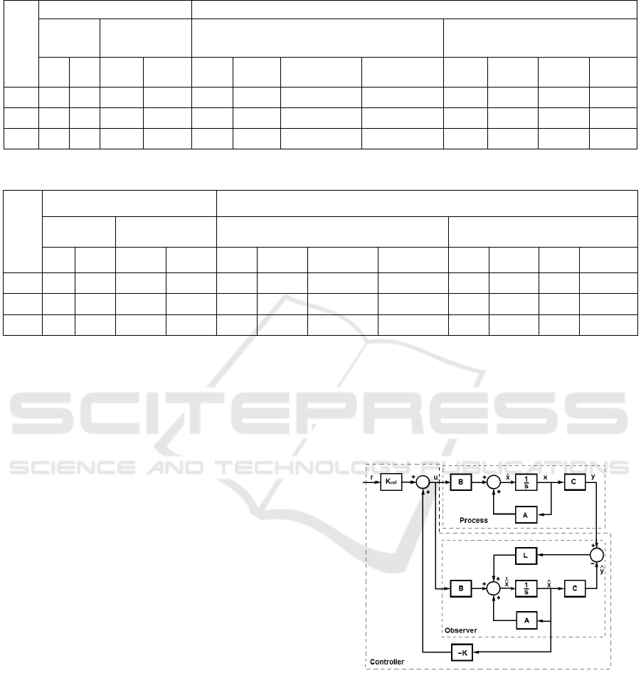
Table 4: Selected poles and state feedback gain matrix parameter values.
i
l
J
Rigid drive dynamics Flexible drive dynamics
Selected
poles
State feedback
gain matrix
Selected poles State feedback gain matrix
*
1
p
*
2
p
1c
k
2c
k
*
1
p
*
2
p
*
3
p
*
4
p
1c
k
2c
k
3c
k
4c
k
1
l
J
-20 -11
0.0313 0.0032 -12.26 -48.49 -28.32+59.33i -28.32-59.33i 0.3234 0.0069 -0.7223 0.0247
2
l
J
-20 -7
0.0321 0.005 -8.33 -26.32 -17.52+38.48i -17.52-38.48i 0.0749 0.0038 -0.103 0.0124
3
l
J
-20 -5
0.0365 0.0079 -4.95 -16.46 -17.38+31.37i -17.38-31.37i 0.028 0.003 -0.015 0.0104
Table 5: Selected poles for the observer and observer gain parameter values.
i
l
J
Rigid drive dynamics Flexible drive dynamics
Selected poles
Observer gain
matrix
Selected poles Observer gain matrix
1o
p
2o
p
1
l
2
l
1o
p
2o
p
3o
p
4o
p
1
l
2
l
3
l
4
l
1
l
J
-220 -121
332.37 23751.6 -36.80 -145.47 -84.96+177.9i -84.96-177.9i 329.8 65168.8 1331
13480.37
2
l
J
-220 -77
291.65 15379.7 -25.06 -78.79 -52.56+115.4i -52.56-115.4i 192.3 23871.9 320.4
2252.13
3
l
J
-220 -55
271.63 11184.6 -14.83 -49.46 -52.16+94.12i -52.16-94.12i 154.1 15181.1 143.3
390.83
By allocating the poles of the observer, the
characteristic polynomial Δ
ob
(s) is expressed as
0
1
1
...)()( 


n
n
n
oob
sspss
(17)
The selected poles for the observer and observer
gain matrix parameter values are given in Table 5.
Because both the system (10) and the observer
(14) have the same order n, the order of the closed
loop system is 2n. In order to obtain the state feedback
observer, the design of the observer as well as the
design of the state feedback can be realized
separately. The closed-loop system is defined as
r
K
ref




























0
~
0
~
B
x
x
CLA
KBKBA
x
x


(18)
Due to the fact that the matrix on the right side
is block diagonal, the characteristic polynomial of the
closed-loop system has the form
). det() det()( CLAIKBAI  sss
xx
(19)
This property is called the separation principle
(Åström and Murray, 2009). A schematic diagram of
the controller is illustrated in Figure 2. It can be
observed that the controller includes a dynamic model
of the plant, thus respecting the internal model
principle. It can also be noticed that the observer
determines the dynamics of the controller. As such,
the controller can be regarded as a dynamical system
having y as input and u as output:
.
, ) (
rKu
y
ref


xK
LxCLKBAx




(20)
The t.f. of the controller has the form


. )(
1
LCLKBAIK

 ssH
c
(21)
Figure 2: Schematic diagram of an observer-based
controller.
4 EXPERIMENTAL RESULTS
The observer-based controller structure was
developed and tested on the mechatronics system –
MIPE220 – with rigid and flexible drive dynamics, in
the framework of position control solutions designed
State Observers for Mechatronics Systems with Rigid and Flexible Drive Dynamics
391

Table 6: Mean Square errors.
Inertia
Rigid drive dynamics Flexible drive dynamics
ref
step
ref
staircase
ref
step
ref
staircase
Sim Exp Sim Exp Sim Exp Sim Exp
1
l
J
5.5161e-06 0.0035 2.2754e-06 0.0014 3.4579e-05 0.0244 1.2967e-05 0.0128
2
l
J
5.3035e-05 0.0041 2.0467e-05 0.0018 6.1088e-04 0.0255 1.6291e-04 0.0137
3
l
J
4.0919e-04 0.0059 1.5566e-04 0.0022 3.5115e-03 0.0737 1.3168e-03 0.0401
for three specific load disk inertia values. The
proposed design approaches were tested and validated
by real-time experimental results. The system’s
responses in two experimental scenarios were
considered: 1. the proposed control solutions
responses were tested first using a step reference and
are illustrated in Figures 3 and 5 and 2. a staircase
change for the reference signal was employed and the
proposed control solutions were tested again on the
time frame of 30s and are illustrated in Figures 4 and
6.
In order to highlight how the specified control
system performance was achieved, a comparative
analysis between simulation and experimental results
is carried out in terms of MSE values included in
Table 6.The values of MSE, considered as a global
performance index, between the real system variable
k
p
and its estimation
k
p

, are defined as (p –
position):
.)(
1
1
2



m
k
kk
pp
m
MSE

(22)
Taking into account the MSE values presented in
Table 6 and the graphs illustrated in Figures 3 to 6, a
set of following conclusions are pointed out: 1) the
motivation to use observers (state observers) is due to
the fact that through the predictive negative reaction,
these design approaches have the advantage of faster
convergence and a reduced sensitivity of estimation
to parameter variation; 2) the controller structure is
identical for systems with one input and one output as
well as for systems with multiple inputs and outputs
with the same form for the controller equations, the
only difference being the fact that the feedback
gain K and the observer gain L are matrices instead
of vectors; 3) the separation principle – for the output
feedback, the eigenvalue assignment can be split into
an observer and a state feedback eigenvalue
assignment – leads to a simplified design; 4) with one
dynamic system both a controller and an observer can
be developed; 5) the proposed approaches offer
contributions for the robustness and dynamic
performance of the system; 6) based on the
comparative analysis it can be concluded that the
proposed design approaches, prove to be viable and
ensure a good reference tracking ability; 7) the use of
these state observers leads to dynamically and
permanently improved performance.
5 CONCLUSIONS
This paper gives details regarding the design and
implementation of state observers designed for three
specific load disk inertia values in order to estimate
the position for a mechatronics system with rigid and
flexible drive dynamics. The proposed design
approaches are validated by means of real-time
experimental results. The graphs illustrated in Figures
3 to 6 proved that these approaches are viable and
ensure a good reference tracking ability. The use of
these observers leads to dynamically and permanently
improved performance.
Future work will investigate further
improvements of the performance indices for the
proposed design approaches. Additionally, optimal
parameter tuning will replace the pole placement
method. Further work will also aim to adapt these
observers to other important cases, through the
extension of the approaches suggested in this paper to
other illustrative applications that include robotics
and autonomous systems (Blažič, 2014; Kovács et al.,
2016), fuzzy models and control (Precup et al., 2018),
engines (Andoga et al., 2018), cognitive models for
prediction and control (Direito et al., 2017; Ferreira et
al., 2017; Braga et al., 2019).
ACKNOWLEDGEMENTS
This work was supported by grants from the Ministry
of Research and Innovation, CNCS - UEFISCDI,
project numbers PN-III-P1-1.1-PD-2016-0331 and
PN-III-P1-1.1-PD-2016-0683, within PNCDI III.
ICINCO 2019 - 16th International Conference on Informatics in Control, Automation and Robotics
392

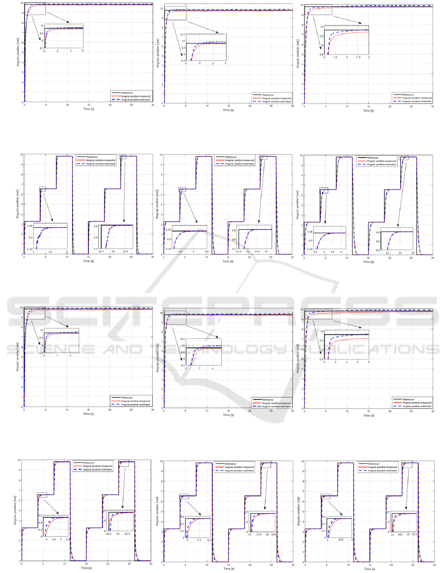
Figure 3: Experimental results concerning the behaviour of observer-based controller designed for MIPE220 with rigid drive
dynamics (step reference): case study 1, 2 and 3.
Figure 4: Experimental results concerning the behaviour of observer-based controller designed for MIPE220 with rigid drive
dynamics (staircase reference): case study 1, 2 and 3.
Figure 5: Experimental results concerning the behaviour of observer-based controller designed for MIPE220 with flexible
drive dynamics (step reference): case study 1, 2 and 3.
Figure 6: Experimental results concerning the behaviour of observer-based controller designed for MIPE220 with flexible
drive dynamics (staircase reference): case study 1, 2 and 3.
State Observers for Mechatronics Systems with Rigid and Flexible Drive Dynamics
393

REFERENCES
Aghannan, N., Rouchon, P., 2003. An intrinsic observer for
a class of Lagrangian systems. IEEE Transactions on
Automatic Control. 48, 936-945.
Andoga, R., Főző, L., Judičák, J., Bréda, R., Szabo, S.,
Rozenberg, R., Džunda, M., 2018. Intelligent situational
control of small turbojet engines. International Journal
of Aerospace Engineering. 2018, paper 8328792, 1-16.
Åström, K. J., Murray, R. M., 2009. Feedback Systems. An
introduction for scientists and engineers. Princeton,
New Jersey, Princeton University Press.
Bishop, R. H., 2007. The Mechatronics Handbook, 2
nd
ed.
Boca Raton, FL: CRC Press.
Blažič, S., 2014. On periodic control laws for mobile robots.
IEEE Transactions on Industrial Electronics. 61 (7),
3660-3670.
Braga, D., Madureira, A. M., Coelho, L., Ajith, R., 2019.
Automatic detection of Parkinson's disease based on
acoustic analysis of speech. Engineering Applications of
Artificial Intelligence. 77, 148-158.
Brown, R. G., Hwang, P. Y. C., 1996. Introduction to
Random Signals and Applied Kalman Filtering, 3
rd
ed.
New York: John Wiley & Sons.
Direito, B., Teixeira, C. A., Sales, F., Castelo-Branco, M.,
Dourado, A., 2017. A realistic seizure prediction study
based on multiclass SVM. International Journal of
Neural Systems. 27 (3), 1-15.
ECP, 2010. Industrial Emulator/Servo Trainer Model 220
System, Testbed for Practical Control Training. Bell
Canyon, CA: Educational Control Products.
Ferreira, R., Graça Ruano, M., Ruano, A. E., 2017.
Intelligent non-invasive modeling of ultrasound-
induced temperature in tissue phantoms. Biomedical
Signal Processing and Control. 33, 141-150.
Gutiérrez-Carvajal, R. E., de Melo, L. F., Rosário, J. M.,
Tenreiro Machado, J. A., 2016. Condition-based
diagnosis of mechatronic systems using a fractional
calculus approach. International Journal of Systems
Science. 47, 2169-2177.
Isermann, R., 2005. Mechatronic Systems: Fundamentals.
Berlin, Heidelberg, New York: Springer-Verlag.
Kovács, B., Szayer, G., Tajti, F., Burdelis, M., Korondi, P.,
2016. A novel potential field method for path planning of
mobile robots by adapting animal motion attributes.
Robotics and Autonomous Systems. 82, 24-34.
Lendek, Z., Babuska, R., De Schutter, B., 2008. Distributed
Kalman filtering for cascaded systems. Engineering
Applications of Artificial Intelligence. 21, 457-469.
Luenberger, D. G., 1966. Observers for multivariable
systems. IEEE Transactions on Automatic Control. 11,
190-197.
Magnis, L., Petit, N., 2016. Angular velocity nonlinear
observer from single vector measurements. IEEE
Transanctions on Automatic Control. 61, 2473-2483.
Marx, B., Koenig, D., Ragot, J., 2007. Design of observers
for Takagi-Sugeno descriptor systems with unknown
inputs and application to fault diagnosis. IET Control
Theory & Applications. 1, 1487-1495.
Precup, R.-E., Teban, T.-A., Albu, A., Szedlak-Stinean, A.-
I., Bojan-Dragos, C.-A., 2018. Experiments in
incremental online identification of fuzzy models of
finger dynamics. Romanian Journal of Information
Science and Technology. 21 (4), 358-376.
Spurgeon, S. K., 2008. Sliding mode observers: A survey.
International Journal of Systems Science. 39, 751-764.
Szedlak-Stinean, A.-I., Precup, R.-E. Preitl, S., Petriu, E.
M., Bojan-Dragos, C.-A., 2016. State feedback control
solutions for a mechatronics system with variable
moment of inertia. In Proc. 13
th
International
Conference on Informatics in Control, Automation and
Robotics, Lisbon, Portugal, 458-465.
Szedlak-Stinean, A.-I., Precup, R.-E., Petriu, E. M., 2017.
Fuzzy and 2-DOF controllers for processes with a
discontinuously variable parameter. In Proc. 14
th
International Conference on Informatics in Control,
Automation and Robotics, Madrid, Spain, 431-438.
Thau, F. E., 1973. Observing the state of nonlinear dynamic
systems. International Journal of Control. 17, 471-479.
ICINCO 2019 - 16th International Conference on Informatics in Control, Automation and Robotics
394