Autonomous Overtaking Maneuver Design based on Follow the Gap

Method

Munire Damla Demir

and Volkan Sezer

AVL Research and Engineering, Istanbul, Turkey

Control and Automation Engineering Department, Istanbul Technical University, Istanbul, Turkey

Keywords:

Collision Avoidance, Motion Planning, Safety, Overtaking, Merging, Autonomous Drive, Highway Driving,

Motion Control, Path Tracking, Stanley Controller, X-sin Function.

Abstract:

This paper proposes a solution for one of the most important components of autonomous driving: "overtaking

maneuver". Follow the Gap method (FGM) is oneof the most popular obstacle avoidance algorithms and

directly obtains steering angle from position of the obstacles around. This paper is the ﬁrst study using FGM

to solve the overtaking problem. Different from previous studies where a trajectory is planned and then a

controller is designed to track it; we use FGM for motion planning and control together. This paper focuses

on overtaking maneuver in a challenging environment like highway trafﬁc where the safety and fast response

are the key factors. After we adapt the FGM to overtaking problem, we compare it with an existing overtaking

method X-sin functions from literature. Since X-sin functions method requires a path tracker (controller),

Stanley method is combined with X-sin functions. At the end of this work, we show several advantages of

FGM comparing to the X-sin functions based overtaking approach.

1 INTRODUCTION

With the rapid development of technology in recent

years, the automotive industry is moving closer to full

autonomous vehicles. The most critical beneﬁt of au-

tonomous driving is human safety. Every year ap-

proximately 1.35 million people die because of traf-

ﬁc accidents according to "Global Status Report on

Road Safety" (Toroyan, 2018). In addition, 25-78%

of accidents happened as a result of driver inatten-

tion (Klauer et al., 2010) and 10% of all crashes hap-

pened during the lane change (G. M. Fitch and Din-

gus, 2009). In order to avoid crashes, one of the most

important thing to do is providing fast response.

Global path planning algorithms requires high

computational time for their operations. For exam-

ple A*, which is one of the most popular graph search

algorithm, ﬁnds a path from point A to B for static

maps (Likhachev and Ferguson, 2009). On the other

hand, it is not very convenient to ﬁnd a new path

using A* if the map changes very often as in dy-

namic environments. D* is introduced as improved

A* which is more adaptable to moving obstacles but

still not as fast as obstacle avoidance methods (Stentz,

1994). Nonholonomic constrains of vehicle are con-

sidered in "Rapidly Exploring Random Tree (RRT)"

method which is a probabilistic approach and pro-

vides a smooth driving (Lavalle, 1998). The main

drawback of these kind of methods is the required

computational time. Moreover, afters suitable trajec-

tory is generated, the trajectory must be followed by

a path tracker algorithm.

The aim of a path tracker algorithm is to calculate

the required control inputs reach from one waypoint

to another. Stanley (Snider, 2009) method and Pure

Pursuit (Coulter, 1992) are two popular tracking al-

gorithms.The comparison of these two approaches is

shown (Cibooglu et al., 2017) which proposes a hy-

brid method at the end. According to the analysis,

Pure Pursuit does not provide a good performance

in cutting roads and Stanley method overshoots at

sharp corners. Another result from analysis is Stan-

ley method has more advantages than Pure Pursuit at

high speeds.

For the solution of overtaking problem, Mixed

Observable Markov Decision Process (MOMDP)

based solution is provided in (Sezer, 2018). However,

this solution is not suitable for real-time applications

due to its computational complexity. Moreover dis-

crete state space representation restricts the operation

of the method. Another overtaking approach X-sin is

proposed in (Zhang et al., 2014) which provides ap-

Demir, M. and Sezer, V.

Autonomous Overtaking Maneuver Design based on Follow the Gap Method.

DOI: 10.5220/0007923502950302

In Proceedings of the 16th International Conference on Informatics in Control, Automation and Robotics (ICINCO 2019), pages 295-302

ISBN: 978-989-758-380-3

295

propriate path using special trigonometric functions.

It requires three main parameters for its operation and

calculation of the path is relatively easy. On the other

hand it still needs a controller algorithm in order to

track the desired path.

Obstacle avoidance algorithms are mostly used for

dynamic environments in order to avoid any obstacle

in a short time. For example bug algorithms (Zohaib

et al., 2013) are based on following the borders of

the obstacles but not useful to implement for high-

way driving and vehicle dynamics. Another obsta-

cle avoidance algorithm is Artiﬁcial Potential Field

Method (Zhu et al., 2006) and (Bounini et al., 2017)

which results smooth steering angles. However, the

tuning parameters can affect the steering angle a lot

and it should be adapted for every situation in high-

way driving while very different scenarios are possi-

ble. Local minimum problem is another critical dis-

advantage of this approach.

Follow the Gap method (Sezer and Gokasan,

2012) is a geometric obstacle avoidance algorithm

for autonomous driving. FGM selects the maximum

gap angle in the ﬁeld of view, it combines the the

goal angle and gap angle considering minimum dis-

tance to obstacle. It also considers the nonholonomic

constraints of the vehicle, does not have local mini-

mum problem and is easy to tune with only one tun-

ing parameter. Improved Follow the Gap (FGM-I)

(Demir and Sezer, 2017) is an extended version of

FGM which solves two drawbacks of original FGM.

FGM-I eliminates chattering effect coming from un-

necessary gap change and chooses goal oriented gaps

in order to ﬁnd a shorter path.

This paper examines the overtaking in highway

conditions where the speed values are relatively high.

Dynamic single track vehicle model is used in order to

obtain more realistic results comparing to pure kine-

matic models (Rajamani, 2011).

In this paper, FGM is implemented as motion

planning and controlling algorithm and compared

with X-sin functions planner and Stanley controller.

Vehicle model, FGM and X-sin planner with Stan-

ley controller (XwS) are explained in section 2, sim-

ulation environment and highway scenarios are ex-

plained in section 3 , and simulation results through

the implementation are shown in section 4. Conclu-

sion of the paper is examined in section 5. Future

Work is provided in section 6.

2 TECHNICAL APPROACH

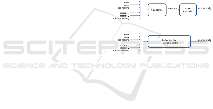
The general approach in autonomous driving is de-

signing a motion planner and a controller as separated

components. As it is shown in Figure 1, X-sin func-

tion as a motion planner generates a collision free path

in accordance with environment (Zhang et al., 2014).

The path is controlled by the Stanley controller which

obtains the steering angle to be given to vehicle model

(Snider, 2009). From now on we call XwS for the

combination of X-sin functions motion planner and

Stanley controller. The principle of operation of X-sin

functions and Stanley method are explained in Sec-

tion 2.3.

The proposed approach is to combine motion

planner and controller using FGM for overtaking ma-

neuver as it is stated in Figure 2. Follow the Gap

method combines motion planner and controller by it-

self so that quick reaction in dynamic environment is

available while considering safety and comfort. The

principle of operation of FGM is explained in Section

2.2.

Figure 1: Concept of Motion Planing and Control using.

Figure 2: Concept of New Approach based on FGM.

2.1 Vehicle Model

In order to make realistic simulations, single track

dynamic vehicle model (Rajamani, 2011) is used in-

stead of a kinematic bicycle model which neglects

tire forces. Even though the kinematic model is ap-

plicable at lower speeds, dynamic model is required

for highway scenarios at high speeds. Since this

work concentrates on overtaking maneuver, longitu-

dinal speed is considered as constant. Dynamic bicy-

cle model is represented as it is shown in Figure 3. X,

Y represent the global coordinates, x, y represent the

local coordinate of vehicle where CG is the vehicle’s

center of gravity. L

is the distance from center of

gravity to front wheel and L

is the distance from CG

to rear wheel. δ and ψ are the steering angle and yaw

angle of the vehicle, respectively. Finally, F

y f

and F

represent the lateral forces.

(1) and (2) are standard equations for lateral dy-

namics. x, y positions of ego vehicle and yaw angle

are obtained by the (2), (3) and (4).

m ˙v = F

y f

cos(δ) +F

+ mv

ψ (1)

ψ = L

y f

cos(δ) −L

(2)

ICINCO 2019 - 16th International Conference on Informatics in Control, Automation and Robotics

296

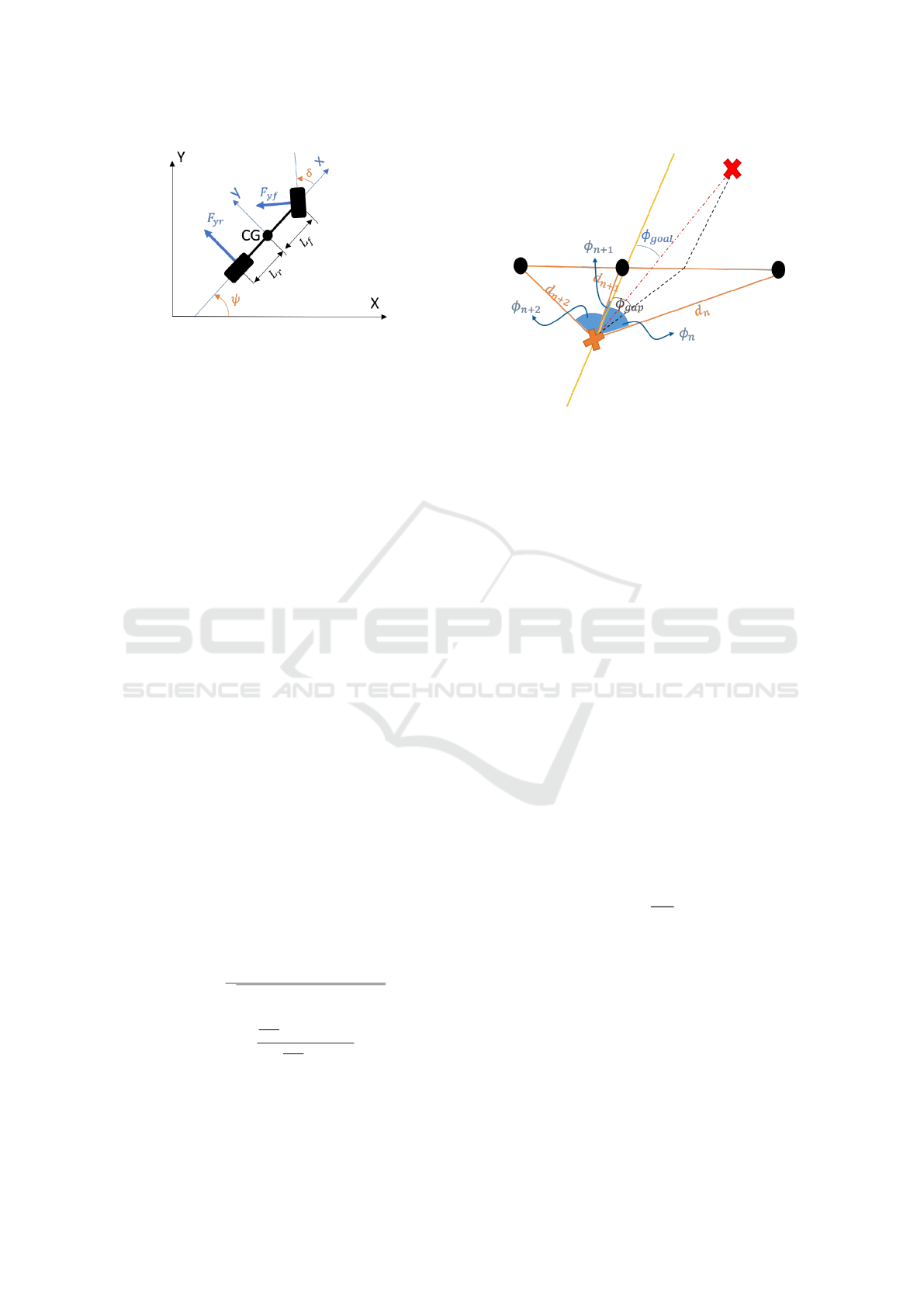
Figure 3: Single Track Lateral Dynamics.

˙x = v

cosψ −v

sinψ (3)

˙y = v

sinψ +v

cosψ (4)

2.2 Follow the Gap Method

FGM basically monitors the maximum gap between

the closest obstacles in ﬁeld of view and generates

a steering angle which avoids the obstacles consider-

ing the goal point (Sezer and Gokasan, 2012). FGM

generates desired heading angle which can be used as

steering angle directly. Figure 4 shows the angles re-

garding to FGM; orange X is the starting point, red X

is the target point, black dots represent obstacles, red

dashed line represents the connection between start-

ing point and goal point, black dashed line represents

the connection between starting point and gap center

of selected obstacles in the ﬁeld of view, d

is the dis-

tance from ego vehicle to the n

obstacle, φ

is the

angle of the n

gap, φ

gap

is the angle of the selected

gap which is developed by the FGM, φ

goal

is the angle

from ego the goal point. (5) calculates φ

gap

in terms

of measurable variables, and (6) provides φ

f inal

which

is the ﬁnal angle for the vehicle. α is a tuning pa-

rameter and selected as 0.5 according to experimental

results. The higher α means the more importance on

gap

so that φ

f inal

is closer to the φ

gap

. The lower α

means the more importance on φ

goal

therefore phi

f inal

is weighted more on φ

goal

. d

min

is the closest distance

from the nearest obstacle which weights φ

goal

and

gap

automatically. According to (6), when the ego

vehicle approaches to an obstacle, φ

gap

is weighted

more than φ

goal

and vice versa.

gap

= cos

−1

n+1

cos(φ

+φ

n+1

)

n+1

+2d

n+1

cos(φ

+φ

n+1

)

− φ

(5)

f inal

min

gap

+ φ

goal

min

+ 1

(6)

f inal

is the desired heading angle but can be di-

rectly used as steering angle as it is implemented in

this paper. For different applications, an additional

Figure 4: Follow the Gap Angle Representation.

controller can be designed to calculate the steering an-

gle in order to get the desired heading angle.

2.2.1 Adaptation of FGM to Overtaking

Maneuver

In order to adapt FGM for overtaking maneuver, we

specify a single goal point that is located in front of

the actor vehicle. This goal point moves with the ac-

tor vehicle. Actor vehicle is also an obstacle for ego

vehicle. The borders of the road are also other obsta-

cles for ego vehicle. If FGM is used as an obstacle

avoidance algorithm to reach the goal point which is

deﬁned in front of actor vehicle, the ﬁnal trajectory

becomes an overtaking maneuver.

The ﬂowchart of overtaking algorithm using FGM

is shown in Figure 5. First, time to collision T

value

is calculated as shown in (7). The algorithm checks

whether that T

value is lower than 2 seconds. This

experimental value is selected according to (Kristofer

D. Kusano, 2011). This ﬁrst part of the approach is

preparation for lane change as shown in Figure 6. In

this ﬁgure, red X is deﬁned as the goal point and blue

dots are obstacles. If T

value is lower than 2 seconds,

the ego vehicle starts lane changing using FGM.

eto

net

(7)

eto

: Distance between ego vehicle to obstacle [m],

: Time to Collision [s], V

net

: Velocity difference

between ego and actor vehicles [m/s]

Secondly, FGM ﬁnds the gap goes forward to the

gap until it reaches the rear left corner of the front

actor vehicle which is shown in Figure 7. This is

the passing phase of overtaking maneuver. Look

ahead range (LAR) distance is added in order to avoid

the quick and dangerous merging so that ego vehicle

keeps its lane until it reaches the location that is de-

ﬁned by LAR.

Autonomous Overtaking Maneuver Design based on Follow the Gap Method

297

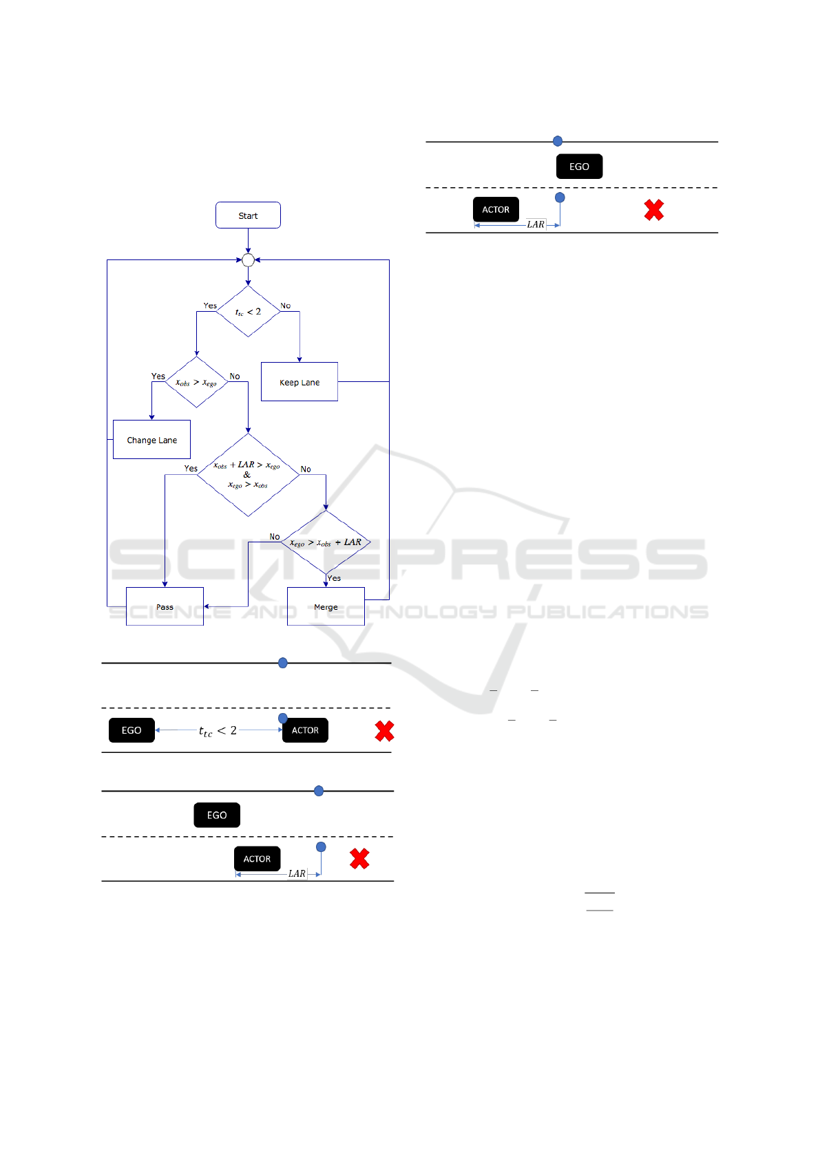
Finally, ego vehicle starts to steer to get back to

the initial lane where LAR away from actor vehicle.

This last phase of overtaking is called "merging" as

shown in Figure 8.

Figure 5: Algorithm of Overtaking.

Figure 6: Lane Change using FGM.

Figure 7: Passing the actor vehicle using FGM.

In section 4, three different speed scenarios are

presented and overtaking performances of FGM are

declared.

Figure 8: Merging using FGM.

2.3 X-sin Function as a Motion Planner

and Stanley Method as a Motion

Controller

2.3.1 X-sin Function as a Motion Planner

X-sin function was developed as a solution for over-

taking maneuver using standard mathematical func-

tions in (Zhang et al., 2014). X-sin is a partial func-

tion which calculates the lateral and longitudinal posi-

tion of the ego vehicle as illustrated in Figure 9. Over-

taking decision is made in the same way as in previous

FGM approach by using (7). Goal position is selected

in the end of the merging distance which dynamically

moves with actor vehicle.

Figure 9 shows the parameters and trajectory of

a typical X-sin function. L

is the distance of lane

changing, O

is deﬁned as distance of passing which

is chosen as the length of the ego vehicle and M

the distance of merging which is selected as same as

Eq. (8) provides the mathematical function of X-

sin where x is the current position and y

is the lane

change distance in y axis.

y(x) =











2π

x −sin



2π

i

x ∈ [0,L

]

x ∈ [L

+ O

]

− y

2π

x −sin



2π

i

x ∈ [L

+ O

+ M

]

(8)

The L

parameter in X-sin is critical for a comfortable

overtaking maneuver. Original paper (Zhang et al.,

2014) proposes an equation which calculates a good

as shown in (9). The maximum allowed acceler-

ation limit a

max

is declared in (Zhang et al., 2014) as

between 1−4m/s

and v

is the longitudinal speed of

the ego vehicle. In this paper, a

max

is selected 3m/s

and L

is calculated according to the vehicle speed v

in section 4. M

is selected same as L

= v

2πy

max

(9)

ICINCO 2019 - 16th International Conference on Informatics in Control, Automation and Robotics

298

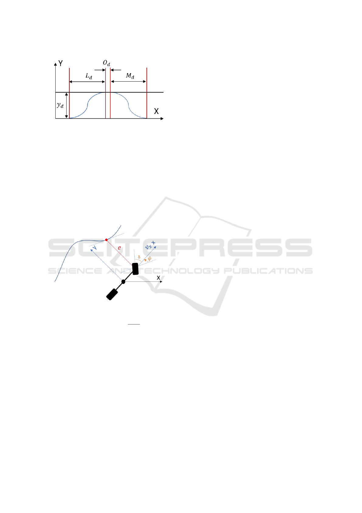
Figure 9: X-sin function representation.

2.3.2 Stanley Method as a Motion Controller

Stanley Method is commonly implemented as a

motion controller for autonomous vehicles (Snider,

2009). In this paper, Stanley method is developed

as a motion controller to track the trajectory which is

generated by X-sin function. Stanley controller cal-

culates the steering angle using yaw error and cross

track error which are represented in (10). Figure 10

illustrates the Stanley method and shows the steering

angle, heading angle, lateral error and longitudinal

speed variables in detail.

Figure 10: Stanley Controller Representation.

δ(t) = ψ(t) +tan

−1



ke(t)

(t)



(10)

Cross track error e(t) is the lateral error which means

the closest distance between the ego vehicle and the

path. Yaw error ψ is the difference between the head-

ing of closest path point and ego vehicle heading, v

longitudinal speed. k is the tuning parameter which is

selected as 10 using trial and error technique in order

to get the best performance.

3 SIMULATION ENVIRONMENT

Matlab/Simulink environment is used to generate ve-

hicle models, to implement algorithms, to create sim-

ulation scenarios, and to compare both of the meth-

ods. The scenarios are selected considering highway

trafﬁc where the speed is between 10 - 35 m/s (KGM,

2018) with 3.5m lane width as it is deﬁned in stan-

dards (EuroTest, 2007).

During simulations, initial positions, initial head-

ing, distance to goal point, environment and limita-

tions are in same manner for both of the methods for

a fair comparison. Goal point is selected as the end of

merging which is represented by M

away from the

actor vehicle. Goal point distance for FGM and XwS

are selected same in the simulations which is calcu-

lated in (9).

4 RESULTS

In this paper, FGM and XwS are compared accord-

ing to different speeds. This comparison is made us-

ing the safety metric, the comfort metric and the total

traveled distance. The related metrics are calculated

using the general norm equation which is shown in

(11). We select p as 2, which means second norm of

the signals are calculated. Similar metrics can be seen

in (Sezer and Gokasan, 2012) and (Demir and Sezer,

2017).

|| f ||



| f (t)|



1/p

(11)

The f (t) function for safety metric is deﬁned as the

distance between the ego and the actor vehicle. It

means that if the distance between ego vehicle and

actor vehicle is generally high, the safety metric re-

sults with higher values in another words this is a

safer overtaking. The f (t) function for comfort met-

ric is deﬁned as the yaw rate of the ego vehicle. The

increase in this metric means that the change ego ve-

hicle’s yaw angle is high which is an uncomfortable

situation for the passenger. Total path is additionally

calculated for comparison.

Figure 11 and Figure 12 illustrates the results of

overtaking for FGM and XwS. The time samples are

added to represent the locations of ego vehicle and

actor vehicle for each speciﬁc time sample.

Table 1 contains a detailed comparison of FGM

and XwS by comfort metric, safety metric and total

traveled path. For both FGM and XwS, the initial

positions are same, goal positions are calculated by

same method and both approaches are compared ac-

cording to the identical speeds. Table 1 shows that, at

the same speeds, both comfort metric and safety met-

ric values of FGM are higher than XwS. The result

of more comfortable and safer overtaking maneuver

is longer paths as shown in Table 1. For example

in Figure 11.a and Figure 12.a, it is clearly seen that,

the total path of FGM is greater than the total path of

Autonomous Overtaking Maneuver Design based on Follow the Gap Method

299

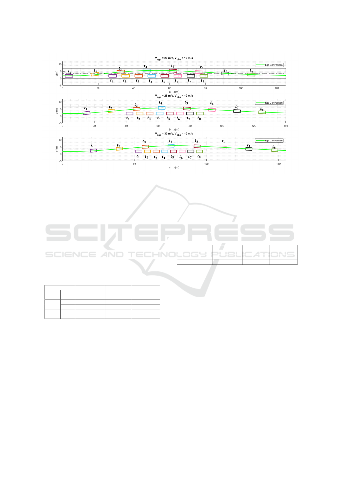
Figure 11: a. Overtaking by FGM at V

ego

= 20m/s, b. Overtaking by FGM at V

ego

= 25m/s, c. Overtaking by FGM at

ego

= 30m/s.

XwS when V

ego

= 20m/s. The longer path of FGM

occurs due to the passing part of overtaking maneu-

ver. During the passing phase, when the ego vehicle

is getting closer to the actor vehicle, d

min

value de-

creases and ego vehicle intends to avoid from actor

vehicle as calculated in (6).

Safer and more comfortable driving of FGM

makes the increase of the total path less important. In

Figure 12.c, the speed of ego vehicle is 30m/s and it

is clearly seen that, Stanley method causes overshoot

in control. This may cause more overshoots when the

speed of ego vehicle is higher.

Table 1: FGM and Comparison Table.

Speed / Metrics Comfort metric Safety metric Total Path [m]

20 m/s

FGM 216.45 21.21 146.84

XwS 333.24 19.37 135.54

25 m/s

FGM 282.34 30.65 161.30

XwS 484.05 25.50 153.77

30 m/s

FGM 371.90 40.16 184.27

XwS 648.70 31.60 174.88

1000 Monte Carlo simulations are implemented to

test FGM and in same environment to calculate the

average improvement rate of FGM. The speed of the

ego vehicle is assigned randomly between 10 - 20 m/s

and the speed of actor vehicle is assigned randomly

between 8 - 12 m/s. Each Monte Carlo simulation is

performed by giving the same random speeds to the

ego vehicle and the actor vehicle for FGM and XwS.

According to the speeds of ego and actor vehicles,

eto

, L

, M

and the goal position are calculated. Av-

erage results of 1000 simulations are shown in Table

According to the results the average comfort met-

ric of FGM is 41% better and the average safety met-

ric of FGM is 13% better than XwS results. On

the other hand, the average total path of 1000 Monte

Carlo simulations of FGM is 2.41% longer which is

the result of safer paths. Overall, FGM is signiﬁ-

cantly safer and more comfortable than XwS and re-

sults with a little bit longer paths.

Table 2: Results of 1000 Monte Carlo Simulations.

Method / Metrics Comfort metric Safety metric Total path [m]

FGM 290.15 31.21 164.02

XwS 493.96 27.01 160.15

Improvement Rate 41% 13% -2.41%

5 CONCLUSION

In this paper, FGM is adapted for overtaking maneu-

ver design and control. After this design, FGM is

compared with XwS in highway overtaking scenarios.

Dynamic single track vehicle model is used for sim-

ulations. One of the main differences between two

approaches is; in XwS we need two separated solu-

tions for planing and control while FGM is enough for

both operations. Monte Carlo results show that FGM

based overtaking solution is 13% safer and 41% more

comfortable than XwS while the total traveled path is

2.41% longer. These results show that FGM is very

suitable to solve the overtaking maneuver.

6 FUTURE WORK

Although FGM is an obstacle avoidance method, it is

observed that it gives better results than XwS at high-

ICINCO 2019 - 16th International Conference on Informatics in Control, Automation and Robotics

300

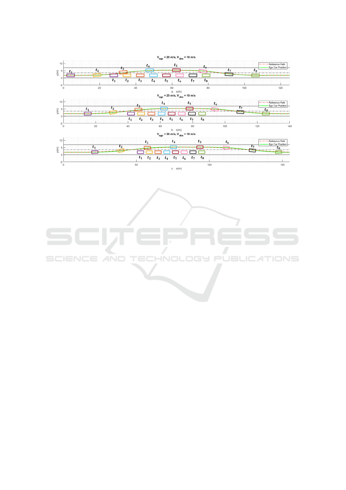
Figure 12: a. Overtaking by XwS at V

ego

= 20m/s, b. Overtaking by XwS at V

ego

= 25m/s, c. Overtaking by XwS at

ego

= 30m/s.

way conditions. The optimization of decision param-

eters for overtaking maneuver such as critical time to

collision value or LAR distance can be thought as a

future study. FGM would be very suitable for dy-

namic environments like urban because of its stability

against moving obstacles. FGM is also easily adapt-

able for intersections, roundabouts or different types

of junctions.

REFERENCES

Bounini, F., Gingras, D., Pollart, H., and Gruyer, D. (2017).

Modiﬁed artiﬁcial potential ﬁeld method for online

path planning applications. pages 180–185.

Cibooglu, M., Karapinar, U., and Soylemez, M. T.

(2017). Hybrid controller approach for an autonomous

ground vehicle path tracking problem. In 2017 25th

Mediterranean Conference on Control and Automa-

tion (MED), pages 583–588.

Coulter, R. C. (1992). Implementation of the pure pur-

suit path tracking algorithm. Technical Report CMU-

RI-TR-92-01, Carnegie Mellon University, Pittsburgh,

PA.

Demir, M. and Sezer, V. (2017). Improved follow the gap

method for obstacle avoidance. In 2017 IEEE Inter-

national Conference on Advanced Intelligent Mecha-

tronics (AIM), pages 1435–1440.

EuroTest (2007). http://www.theaa.com/public_affairs/

reports/eurotest-motorway-roadworks-2007.pdf.

G. M. Fitch, S. E. Lee, S. K. J. H. J. S. and Dingus, T.

(2009). Analysis of Lane-Change Crashes and Near-

Crashes. National Highway Trafﬁc Safety Adminis-

tration.

KGM (2018). Hizsinirlari. http://www.kgm.gov.tr/Sayfalar/

KGM/SiteTr/Traﬁk/HizSinirlari.aspx.

Klauer, S., Guo, F., Sudweeks, J., and Dingus, T. (2010). An

analysis of driver inattention using a case-crossover

approach on 100-car data.

Kristofer D. Kusano, H. G. (2011). Method for estimating

time to collision at braking in real-world, lead vehicle

stopped rear-end crashes for use in pre-crash system

design. SAE International.

Lavalle, S. M. (1998). Rapidly-exploring random trees: A

new tool for path planning. Technical report.

Likhachev, M. and Ferguson, D. (2009). Planning long dy-

namically feasible maneuvers for autonomous vehi-

cles. The International Journal of Robotics Research,

28(8):933–945.

Rajamani, R. (2011). Vehicle Dynamics and Control. Me-

chanical Engineering Series. Springer US.

Sezer, V. (2018). Intelligent decision making for overtaking

maneuver using mixed observable markov decision

process. J. Intellig. Transport. Systems, 22(3):201–

217.

Sezer, V. and Gokasan, M. (2012). A novel obstacle avoid-

ance algorithm: "follow the gap method". Robot. Au-

ton. Syst., 60(9):1123–1134.

Snider, J. M. (2009). Automatic steering methods for au-

tonomous automobile path tracking.

Stentz, A. (1994). Optimal and efﬁcient path planning for

partially-known environments. In Proceedings of the

1994 IEEE International Conference on Robotics and

Automation, pages 3310–3317 vol.4.

Toroyan, T. (2018). Global status report on road safety.

page 2.

Zhang, S., Liu, W., Li, B., Niu, R., and Liang, H. (2014).

Trajectory planning of overtaking for intelligent vehi-

cle based on x-sin function. In 2014 IEEE Interna-

tional Conference on Mechatronics and Automation,

pages 618–622.

Zhu, Q., Yan, Y., and Xing, Z. (2006). Robot path planning

based on artiﬁcial potential ﬁeld approach with sim-

Autonomous Overtaking Maneuver Design based on Follow the Gap Method

301

ulated annealing. Sixth International Conference on

Intelligent Systems Design and Applications, 2:622–

627.

Zohaib, M., Pasha, S. M., Javaid, N., and Iqbal, J. (2013).

Intelligent bug algorithm (iba): A novel strategy

to navigate mobile robots autonomously. CoRR,

abs/1312.4552.

ICINCO 2019 - 16th International Conference on Informatics in Control, Automation and Robotics

302