
A Species-specific Individual-based Simulation Model of Mixed
Mangrove Forest Stands
Ian Estacio
1 a
, Khristoffer Ryan Quinton
1 b
, Edgardo Macatulad
1 c
and Severino Salmo
2 d
1
Department of Geodetic Engineering, University of the Philippines Diliman, Quezon City, Philippines
2
Department of Environmental Science, Ateneo de Manila University, Quezon City, Philippines
Keywords: Mangroves, Simulation, Individual-based, Environmental Modelling, Forest Stand, Salinity, Shading, FON.
Abstract: A species-specific spatially explicit individual-based model has been developed to simulate the development
of mixed mangrove forest stands featuring eight species. The model is a forest stand model that forecasts
mangrove forest development in a 50 m x 50 m plot by simulating the recruitment, growth, and mortality of
individual mangrove trees. Species-specific growth rates, shade responses, and salinity responses of each
species were incorporated to observe differences in forest structure given different salinity conditions. The
model used a modified Field of Neighborhood (FON) approach that considers species-specific responses to
shading and a salinity response function that considers the species-specific salinity upper boundary value of
optimum growth and maximum porewater salinity of a mangrove. Simulation results of 300 years given
salinity conditions in a specific site in Katunggan It Ibajay (KII) showed matching dominant species in the
site. Simulation results of 500 years given extreme low and high salinity values showed consistent forest
dynamics where above-ground biomass and tree count approach certain limit values as the forest stand
matures. Simulation results also of 300 years given salinity values ranging from 1 – 37 ppt showed the
different dominant species for different salinity conditions.
1 INTRODUCTION
The Philippines is one of the countries that hold the
most diverse species of mangroves, having at least
50% of the mangrove species of the world’s
approximately 65 species (Garcia et al., 2013). To
conserve the mangrove biodiversity in the country,
several rehabilitation efforts have already been
conducted in the past. Unfortunately, some have
failed due to lack of knowledge on the ecology
surrounding mangrove forests. To ensure that
conservation efforts are successful, simulation
models of mangrove forests are developed to predict
the outcome of such efforts.
Mangrove forest models depict the dynamics
occurring within mangrove forests. It simulates the
recruitment (dispersal of seedlings), growth, and
mortality (dying) of individual mangrove trees to
forecast the development of the forest as a whole.
Having a mangrove forest model can explain the
a
https://orcid.org/0000-0003-4547-400X
b
https://orcid.org/0000-0003-1837-2673
c
https://orcid.org/0000-0001-7977-2932
d
https://orcid.org/0000-0001-6807-4397
effects of different environmental scenarios to the
survival and conservation of mangrove forests.
There are several types of mangrove forest models
developed. The most common type is the stand
model, which simulates a mangrove forest in a
relatively small area (less than 1 hectare). This type
of forest model simulates different environmental
conditions to analyze the effect of these conditions on
the development of forests.
This paper aims to develop a model for simulating
mixed mangrove forest stand dynamics. The model
features a 50 m x 50 m plot where the growth of
different mangrove species will be simulated given
different environmental conditions. Development of
the model was implemented using the AnyLogic 8.2.4
University simulation software.
Along with the development of the mangrove
forest stand model, this paper also aims to conduct
simulation experiments to demonstrate forest
dynamics, to test species dominance at different
Estacio, I., Quinton, K., Macatulad, E. and Salmo, S.
A Species-specific Individual-based Simulation Model of Mixed Mangrove Forest Stands.
DOI: 10.5220/0007925701530164
In Proceedings of the 9th International Conference on Simulation and Modeling Methodologies, Technologies and Applications (SIMULTECH 2019), pages 153-164
ISBN: 978-989-758-381-0
Copyright
c
2019 by SCITEPRESS – Science and Technology Publications, Lda. All rights reserved
153

salinity conditions, and to apply the model in a
sample test site.
2 INTEGRATION OF CURRENT
MODELS
Several mangrove forest stand models have already
been developed simulating different scenarios to
answer ecological questions regarding mangrove
forests.
One of the most famous mangrove stand models
developed is the FORMAN model (Chen and
Twilley, 1998). This model is famous for featuring a
mixed forest stand (a forest stand with more than one
species) with mangrove species having species-
specific responses to different environment factors.
The FORMAN model is also a gap dynamic model,
meaning it features a plot with rows and columns of
cells called gaps (500 m
2
each). In the model, a tree
occupies a gap but its location within the gap is not
specified. Just like most mangrove stand models, each
tree is described by its diameter at breast height
(DBH) and height. Trees compete with other trees by
the amount of light received by a tree within the gap,
meaning the highest tree within the gap experiences
maximum growth while the trees below experience
hindered growth depending on the amount of light
they receive. Trees respond to their environment
based on the conditions within the gap. One of the
disadvantages of this model is that the locations of
trees are not explicitly defined in space; they are just
defined as located in a specific gap. This makes
modelling of spatially-explicit processes difficult.
This problem was addressed by the model KIWI
(Berger and Hildenbrandt, 2000). In this model, the
mangrove trees are explicitly defined in space, with
each tree having x and y coordinates along with its
DBH and height. Trees compete with each other
through the Field of Neighborhood (FON) approach,
where the growth of each tree is hindered by
neighboring trees. The magnitude of how a tree’s
growth is hindered is dictated by the size, proximity,
and number of neighboring trees. Trees respond to
their environment by sensing the environmental
conditions in their location. One of the disadvantages
of this model is that light reaching an individual tree
is not calculated as the FON approach already
considers light availability as part of the competition
computed. Hence, the species-specific responses of
the mangroves to shading cannot be considered. It is
important that species-specific shade-tolerance of
each tree is considered as this significantly affects
their growth (Dangremond et al., 2015).
Another mangrove forest model is the SEHM
model (Jiang et al., 2012). The SEHM model also
features a mixed stand but is composed of mangrove
and hammock trees. Environment responses are not
species-specific and is based on the general responses
of the trees. The model aims to explain what causes
the ecotones which separate the zonation of the two
tree types. A unique feature of this model is its
dispersal process. Unlike the other models where
seedlings are placed in random locations in the plot,
the SEHM model takes into account the proximity of
the seedlings to its parent tree; seedlings have higher
probability of being established nearer to its parent
tree and a limit is set to how far seedlings can be
established from the mother tree. Different types of
trees have different limits of dispersal hence the
species-specific dispersals of trees can be considered.
Another latest model is the mesoFON model
(Grueters et al., 2014). The main feature of this model
is the plasticity of each individual tree’s trunk,
meaning the trunk can bend in angles depending on
nearby competition from other trees. A unique feature
of this model is that it breaks down the Field of
Neighborhood (FON) into above- and below-ground
components, each signifying the competition for light
and below-ground resources, respectively. This paves
way to the possibility of using FON and species-
specific responses to light availability at the same
time.
3 STUDY AREA
The study area is the Katunggan It Ibajay (KII)
Mangrove Eco-park in Aklan, Philippines. KII Eco-
park was chosen because of its rich diversity of
mangrove species and the availability of site data.
Data from different Philippine research projects
were acquired for the simulation. Point shapefile of
samples of mangrove trees in KII (Figure 1) were
acquired from the Mangrove Remote Sensing
(MaRS) project of the IAMBlueCECAM program.
The point shapefile contains data of the species name
and explicit location of the trees. Orthophoto of the
area with spatial resolution of 6 cm was also acquired
from the same project. Salinity raster files with spatial
resolution of 10 m were acquired from the
Hydrodynamic Modelling for the Assessment of
Protective Services of Mangroves and Seagrass
(HMAPS-MS) project of the IAMBlueCECAM
program.
SIMULTECH 2019 - 9th International Conference on Simulation and Modeling Methodologies, Technologies and Applications
154
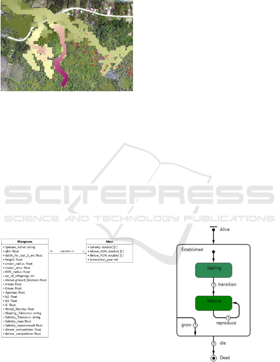
Figure 1: Orthophoto of the KII Eco-park overlayed with
salinity raster file (pixels of color closer to red have lower
salinity while pixels closer to green have higher salinity)
and tree point shapefile (points colored based on species).
4 MANGROVE FOREST STAND
MODELLING
Modelling of the mangrove forest stand was
implemented through the AnyLogic 8.2.4 University
simulation software. Two agents are present in the
model: the Main agent which represents the
environment and the Mangrove agent which represent
the individual mangrove trees (Figure 2). The time
step of the simulation is one year. Spatial extent was
chosen to be a square plot of 50 m x 50 m to
accommodate areas in the forest where the salinity
data only has width of about 50 m.
Figure 2: Class diagram of the mangrove forest stand
model.
4.1 Main Agent
The Main agent, or the environment agent, holds the
variables, parameters, functions, other agents, and
visualization for describing the environment of the
simulation. This includes the initialization, the plot,
and the conditions.
For the model, the environment variables
considered is salinity. Parameters accepted are the
initial number of saplings and the initial conditions of
the environment. Three views can be accessed in the
simulation window: 2D view, 3D view, and Statistics
view.
4.2 Mangrove Agent
Each mangrove agent represents an individual
mangrove tree. The mangrove agent follows a
statechart which describes how the agent follows the
three main processes: recruitment, growth, and
mortality (Figure 3).
An individual mangrove has a state of either
sapling or mature. Saplings are mangrove trees that are
still incapable of producing seedlings while matures
can already reproduce. Transition from sapling to
mature happens once the DBH of an individual tree has
exceeded 1/15
th
of its maximum DBH (D > D
max
/15).
The growth of an individual mangrove depends on its
conditions such as competition from other trees and
environmental factors at the site. Death occurs if the
average annual growth of a tree for the last 5 years is
less than half of its average growth rate (∆D
last5yrs
<
0.5*D
max
/Age
max
), which happens due to aging or
environmental conditions (Berger and Hildenbrandt,
2000).
Figure 3: The statechart of the mangrove agent. Processes
represented by a clock icon are executed every time step
while processes represented by a question mark icon are
executed only when specific conditions become true.
A Species-specific Individual-based Simulation Model of Mixed Mangrove Forest Stands
155
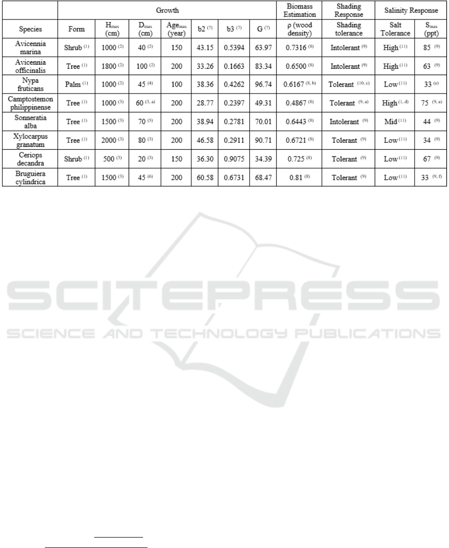
Table 1: Species-specific parameters for each of the eight species in the model.
(1)
Duke et al. (1998),
(2)
FAO Ecocrop (2018),
(3)
Giesen et al. (2007),
(4)
CABI (2018),
(5)
Bojo (1995),
(6)
Madani and Wong (1995),
(7)
Botkin
et al. (1972),
(8)
World Agroforestry (n.d.),
(9)
Smith (1992),
(10)
Ma et al. (2015),
(11)
Reef and Lovelock (2015),
(a)
Assigned from the parameter of Camptostemon schultzii,
(b)
Assigned from the wood density of Palma cocos Miller,
(c)
Assigned from the
properties of Palms in general,
(d)
Assigned from the estuary location of Camptostemon schultzii,
(e)
Assigned from field data,
(f)
Assigned from
the properties of Bruguiera sexangula.
4.3 Gathering and Assignment of
Species-specific Parameters
Eight mangrove species listed in the tree point
shapefile of the study site were considered in the
model (Table 1). These species have species-specific
parameters which dictate their unique growth,
biomass, and environmental response patterns. To
assign the specific parameters of these species,
different literatures were reviewed to gather the
properties of these species. For the assignment of the
Age
max
, the species’ form was used as basis. The
Age
max
is 100 years for palms, 150 years for shrubs,
and 200 years for trees. Growth parameters b2 and b3
control the species’ allometry while parameter G
control the growth rate.
4.4 Growth
The model adopts the growth function for optimal
conditions with reduction factor as provided in the
FORMAN model (Chen and Twilley, 1998). Overall
growth of a tree is represented by the yearly increase
of the DBH, ∆D (cm), which is computed as follows:
(1)
where D is the tree’s DBH (cm), H is the tree height
(cm), and f
red
is the reduction factor in growth due to
environmental conditions. The reduction factor,
which has a value range from 0 to 1, is composed of
the tree’s response to salinity and the combined above
and below competition between trees, expressed as:
(2)
where S is the salinity response and C is the combined
above and below competition response. These factors
also have a value range from 0 to 1. Lower values for
these factors lead to lower growth for the tree.
Tree height (cm) is computed as follows (Berger
and Hildenbrandt, 2000):
(3)
Crown radius (cm), r
crown
, is computed as shown
below (Berger and Hildenbrandt, 2000). The crown
area (m
2
), A
crown
, is just a circle with radius r
crown
.
(4)
The Radius of Field of Neighborhood (cm), r
FON
,
is assigned as a proportion of the r
crown
. In this model,
the coefficient assigned is 1.5, as follows:
(5)
4.5 Recruitment
The number of saplings established in the plot per
year depends on the number of seedlings produced by
each tree and the environmental conditions present
for the seedlings to completely turn to a sapling.
The number of seedlings, N
seed
, produced per
mangrove tree is computed as follows below
(Grueters et al., 2014). The constant 0.5 was assigned
SIMULTECH 2019 - 9th International Conference on Simulation and Modeling Methodologies, Technologies and Applications
156

so that a sufficient number of saplings are established
for gaps in the forest stand.
(6)
The position of where an individual seedling will
be established is randomly determined around the
parent tree. The distance from the parent tree is given
by the distance probability distribution, dis(d), as
follows (Jiang et al., 2012):
(7)
where d is the distance from the parent tree. The
probability of the seedling surviving to become a
sapling, P
sap
(x,y) in location (x,y) is given by the
following (Berger and Hildenbrandt, 2000):
(8)
where F(x,y) is the total Field of Neighborhood
(FON) on the location due to competition. Once it is
determined that a seedling will survive to become a
sapling, a sapling will be established on the subject
location with a DBH of 1.27 cm (Chen and Twilley,
1998).
This recruitment process provides stochasticity in
the model and implies that different positions,
number, and species of saplings are established at a
certain area given different simulation runs.
4.6 Mortality
The model adopts the mortality process of the KIWI
model where the probability of dying of a tree
increases after continuous periods of growth
depression (Berger and Hildenbrandt, 2000). Growth
depression may be due to two factors: environmental
stress and age.
Environmental stress may be due to exposure to
harsh environmental conditions such as high salinity
or low light availability due to shading.
Environmental stress is signified by the reduction
factor f
red
. Growth depression due to age happens
based from the growth function. As a tree reaches its
maximum DBH (or maximum age), its growth
decreases until the growth increment reaches 0.
When the average annual growth of a tree for its
last five years, ∆D
last5yrs
, is less than half of the
average annual diameter growth (∆D
last5yrs
< 0.5 *
D
max
/Age
max
), the tree dies and leaves the plot.
4.7 Above-ground Biomass Estimation
The above-ground biomass of an individual tree (kg),
BIOM, is computed by using the biomass allometry
equation that uses the wood density of a tree
(Komiyama et al., 2008), as shown below. Since
different species have different wood densities,
different above-ground biomass will be computed for
different species given the same DBH.
(9)
4.8 Salinity Response
The salinity response, S
r
, is computed using a
submodel that considers the upper boundary value of
optimum growth and maximum porewater salinity of
a mangrove species. The submodel is given by the
following:
(10)
where S
UOG
is the assigned upper boundary salinity
value for optimum growth and S
max
is the species-
specific maximum porewater salinity. S
UOG
is
assigned per species based on its Salinity Tolerance
from Table 2.
Table 2: Salinity upper boundary values for optimum
growth for each salinity tolerance.
Salinity Tolerance
S
UOG
Low
25
Mid
30
High
40
The salinity response equation was formulated so
that the growth of a mangrove exponentially decays
along a specific salinity gradient. At salinity values
less than the S
UOG
(or the salinity values for optimum
growth), the salinity response is 1 for there is no
reduction in growth. At salinity values greater than
the S
UOG
, the salinity response decreases
exponentially until it becomes 0 at the salinity value
of S
max
, where the mangroves species cannot survive.
4.9 Competition between Mangrove
Agents
At radius r (cm) from the center of the tree, the
intensity of Field of Neighborhood (FON) exerted by
a tree to signify its competition strength is given by
(Berger and Hildenbrandt, 2000):
(11)
where r
trunk
is the radius of the trunk (cm) which is just
half of the DBH, and I
max
and I
min
are competition
A Species-specific Individual-based Simulation Model of Mixed Mangrove Forest Stands
157

constants (Table 3). FON was divided into above and
below ground components to signify competition for
light and below-ground resources availability,
respectively (Grueters et al., 2014). Different I
max
and
I
min
are used for above and below competition. The
assigned I
max
values mean that above competition
(light availability) affects the growth of an individual
tree significantly more than the below competition
(below-ground resources availability). An I
min
value
close to 1 for below competition means that FON
value is almost constant from trunk to the edge of the
Field of Neigborhood. Meanwhile, an I
min
value of
0.07 for above competitions means FON value
decreases drastically at an exponential rate from trunk
to the edge of the Field of Neigborhood.
Table 3: Values for I
max
and I
min
for above and below
competition.
Competition part
I
max
I
min
Above
competition
0.95
0.07
Below
competition
0.05
0.999
The total competition experienced per k
th
tree,
Compet, is obtained using the following equation
(Berger and Hildenbrandt, 2000):
(12)
This means that the sum of all FON (from
neighboring trees except the tree itself) over the area
within the Field of Neighborhood is the total
competition. Since the FON was separated into above
and below parts, the total competition also has
Compet
above
and Compet
below
parts.
To obtain the competition response, the species-
specific shading tolerance of the tree was considered.
Equations from FORMAN (Chen and Twilley, 1998)
were modified to accommodate the above
competition concept. Since Rhizophora mangle was
used in mesoFON, the shade tolerant response (the
growth-reduction factor of Rhizophora mangle in
FORMAN) is equivalent to the competition response
(the growth-reduction factor used for Rhizophora
mangle in mesoFON). The shade tolerant response,
L
shadetolerant
is equated with the competition response,
as given below:
(13)
By rearranging the shade tolerant response
equation in FORMAN, the available light, AL, is
acquired as follows:
(14)
Since available light is already computed, the
shade intolerant response for shade intolerant species,
L
shadeintolerant
can be acquired by using the original
equation from FORMAN.
(15)
The Above Competition response, C
above
, of a
mangrove is adopted from the light responses based
on the species-specific response to shade of the tree.
If the mangrove species is shade tolerant, C
above
=
L
shadetolerant
; if it is shade intolerant, C
above
=
(L
shadeintolerant
+ L
shadetolerant
)/2.
The total competition response is computed using
the equation below:
(16)
5 SIMULATION EXPERIMENTS
Three simulation experiments were conducted to
verify the dynamics and results of the model. For all
experiments, 120 saplings, with 15 saplings per
species and with DBH of 1.27 cm, were placed
around the plot at the start of each simulation.
Saplings were placed such that there is as much space
from each other as much as possible. This
initialization setting simulates an environment where
a bare area is planted with saplings and as time
progresses, a forest pattern with specific dominating
species arises depending on the salinity condition of
the area.
5.1 Validation of Site Species
Dominance Experiment
The first model experiment used simulations to see if
the simulation results of species dominance given
actual site salinity data matches the actual species
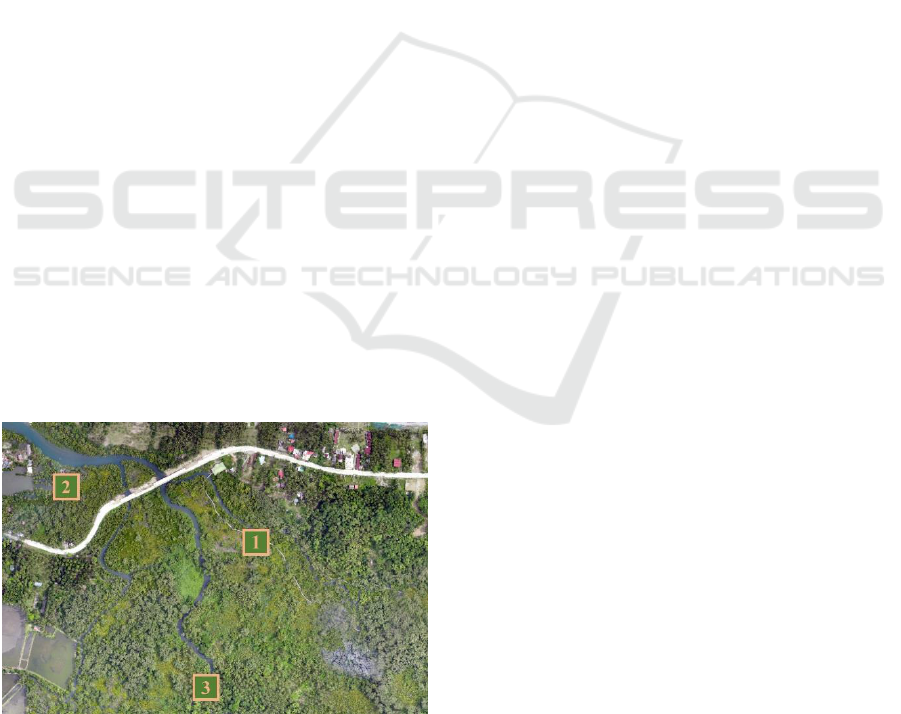
dominance in the site. For this experiment, a test site
in KII which contains parts of the tree point shapefile
was chosen (Figure 4). This test site, named Test Site
1, is quite upstream from the estuary but still has a
high average salinity value of 25.91 ppt.
For this experiment, 10 replications of 300-year
simulation runs were executed. 300 years was used as
this is the forest stand age where the second
generation of trees are already dominating (Bormann
and Likens, 1979). The annual median total above-
ground biomass (AGB) of each species for the 10
replications were acquired. Median was used instead
SIMULTECH 2019 - 9th International Conference on Simulation and Modeling Methodologies, Technologies and Applications
158
of mean as the distribution of values of the AGB for
10 replications were not normally distributed,
specifically skewed to the right.
The median AGB values from the simulations
were then classified into dominance levels through
the Jenks natural breaks optimization using the R
programming language. The dominance level of the
species at the site were also classified based on the
species tree count from the shapefile. The dominance
levels from the simulation and the site were then
compared to see if the dominance level per species
matches.
5.2 Mangrove Forest Development
Experiment
The second model experiment used simulations to see
how a mangrove forest stand develops as the forest
stand ages. Two indicators were used to quantify the
annual development of the forest stand: the total
above-ground biomass (AGB) and the total tree count
in the forest (N). For both indicators, only trees who
have reached the mature state were considered in the
calculations.
Two test sites in KII were chosen such that sites
have relatively different salinity values. Test Site 2 is
near the opening of the estuary in KII eco-park with
average salinity value of 13.50 ppt. Test Site 3 is
farther upstream from the estuary with average
salinity value of 30.241.
For every site, 10 replications of 500-year
simulation runs were executed. The annual mean total
AGB and annual mean total tree count for the 10
replications were acquired. Annual standard
deviation of the two indicators were also noted. From
the values acquired, analysis was done.
Figure 4: Test sites simulated in KII Eco-park. Test Site 1
was used in the first experiment while Test Sites 2 and 3
were used in the second experiment. Test Sites 1, 2, and 3
have average salinity values of 25.91 ppt, and 30.24 ppt,
13.50 ppt, respectively.
5.3 Species Dominance Vs Salinity
Experiment
The third model experiment used simulations to
understand the influence of different salinity values to
the dominance of mangrove species given that they
were all planted as saplings at the start of simulation.
Different simulation runs were executed, varying the
salinity values from 1 ppt to 37 ppt with an interval of
3 ppt. 1 ppt was used as the minimum value as
mangroves generally dominate in saline areas and
they are outcompeted by terrestrial trees in freshwater
areas. 37 ppt was used as the maximum value as 35
ppt is the average salinity value of seawater and a
little leeway was given for values exceeding the
average.
Per salinity value, 10 replications of 300-year
simulation runs were executed. In each simulation,
the subject salinity value was placed constant
throughout the whole plot. After the 300
th
year of
every simulation, the dominance of each species
represented by their total AGB was examined. The
median total AGB for the 300
th
year for every species
for the 10 simulations was computed. The median
AGB values in reference to per species and per
salinity value were analyzed.
6 RESULTS AND DISCUSSION
6.1 Visualization of the Mangrove
Forest Stand
The visualization of the mangrove forest stand is
available in 2D (POV from the sky) and 3D (Figure
5). Resulting simulation runs show that trees are
spaced enough such that the canopies don’t overlap
too much. Canopies of the tallest trees tend to cover
almost the whole forest floor. This is in line with
structures observed in forests where the tallest trees
cover the forest floor, limiting the available light
passing through top-most canopy. In effect, trees that
are in the top-canopy are dominant in size as they
don’t experience hindered growth.
Based from observation of the visualized
mangrove forest stand, forest gap dynamics is
followed, where saplings establish only at locations
where there is available light or no above canopy.
Even if a sapling was to successfully establish at
locations with above canopy, it dies in about 1 or 2
years.
When a top-canopy tree dies, saplings immediately
establish in the area of the deceased tree.
A Species-specific Individual-based Simulation Model of Mixed Mangrove Forest Stands
159
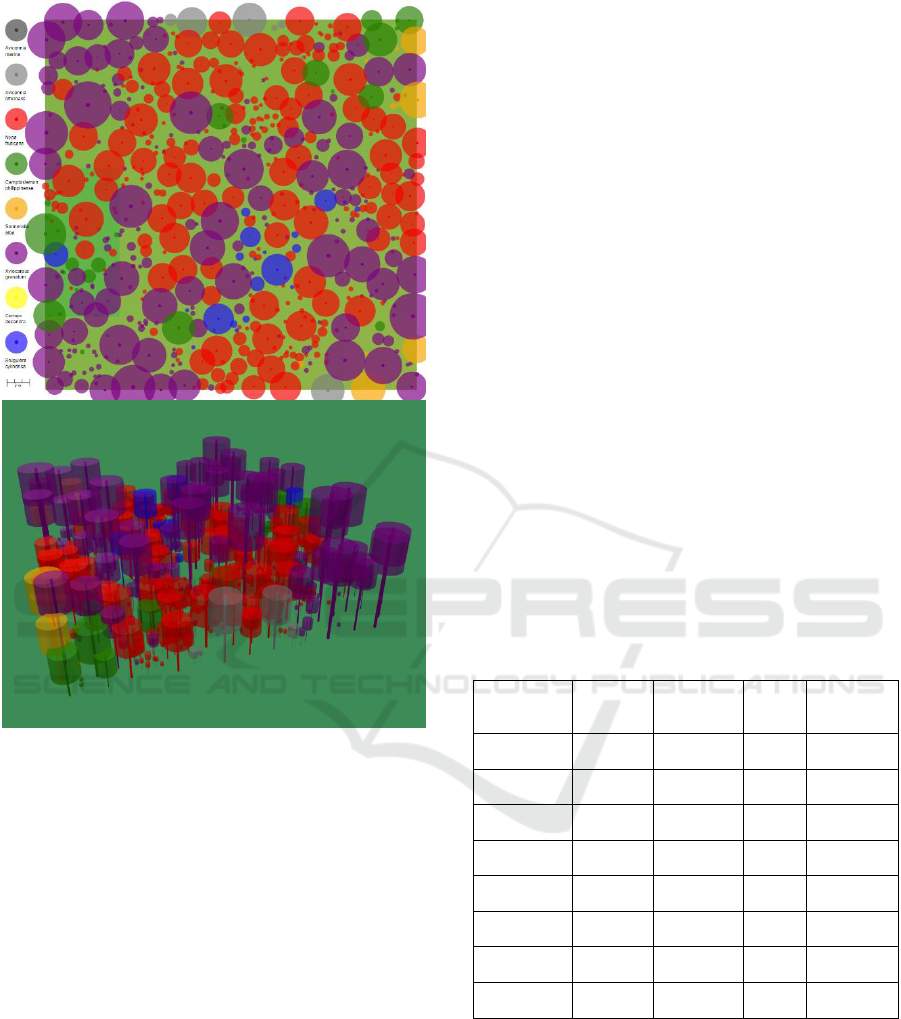
(a)
Figure 5: Visualization of the mangrove forest stand. (a) 2D
view with POV from the sky; (b) 3D view.
This also follows the concept of gap dynamics
where when a tree dies, it paves way for new trees to
dominate.
6.2 Validation of Site Species
Dominance
From simulation runs of Test Site 1, the dominance
curves of species in relation to the forest stand age
was derived (Figure 6). Throughout all years, the
dominance of species with respect to each other was
almost the same. Avicennia officinalis was the most
dominating species in the mangrove forest stand.
Sonneratia alba, Xylocarpus granatum, and
Camptostemon philippinensis were also dominant but
in lower numbers. Avicennia Marina, Nypa fruticans,
Ceriops decandra, and Bruguiera Cylindrica were
just out-dominated.
The median AGB values of the eight species at the
300
th
year were classified into three classes through
the Jenks natural breaks optimization method using
the R programming language. The three resulting
classes were classified as dominance levels of High,
Mid, and Low values (Table 4).
From the tree point shapefile of KII Eco-park,
dominance levels of the species at the site were
classified based on the number of trees that have been
counted per species (Table 4). Jenks natural breaks
optimization method was also used.
Comparing the dominance levels of the mangrove
species in the field to the results of the simulation, six
of the eight species matched, with Avicennia
officinalis matching in high dominance, Xylocarpus
granatum matching in mid dominance, and Avicennia
marina, Nypa fruticans, Ceriops decandra and
Bruguiera cylindrica matching in low dominance.
The simulation results for the other two species
Camptostemon philippinense and Sonneratia alba,
were not far from the field data as the results were
only one level different.
From the results of this experiment, the model
may be ready to be used to assess the effectiveness of
a mangrove reforestation effort given that the species
to be used for planting and the salinity conditions in
the site is known.
Table 4: Comparison of the simulated dominance level and
the site dominance level per species.
Species
AGB at
300
th
year
Simulated
dominance
level
Site
tree
count
Site
dominance
level
Avicennia
marina
453
Low
9
Low
Avicennia
officinalis
164711
High
31
High
Nypa
fruticans
916
Low
7
Low
Camptostemon
philippinense
24915
Mid
6
Low
Sonneratia
alba
22211
Mid
6
Low
Xylocarpus
granatum
18142
Mid
20
Mid
Ceriops
decandra
0
Low
3
Low
Bruguiera
cylindrica
0
Low
9
Low
6.3 Mangrove Forest Development
From the simulation runs of two test sites in KII,
forest development trends were observed for a 500-
year period (Figure 7). As the forest stand ages, the
above-ground biomass in the forest stand approaches
a limit. This observation in forest dynamics is
consistent with the biomass development model
(b)
SIMULTECH 2019 - 9th International Conference on Simulation and Modeling Methodologies, Technologies and Applications
160
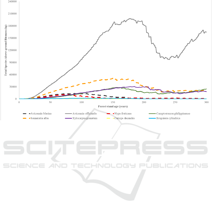
Figure 6: Dominance of eight species in KII Eco-park over a 300 year-period in Test Site 1.
Bormann and Likens, 1979; Keeton et al., 2011). In
the model, it states that there will be peaks in the
biomass of a forest stand in less than 200 years. In the
case of the mangrove forest simulation model, the
peak in biomass accumulation happens around after
150 years. The biomass development model also
states that after the biomass peak, a period of a
decreasing biomass happens. This is due to the dying
of the first generation of mangrove trees. After this
decline in biomass, a steady-state biomass is observed
where the biomass of the forest approaches a certain
limit. The biomass trend will increase and decrease
around this limit value due to dying of dominant trees
and growth of new dominant trees.
The count of individual mature trees also reaches
a limit as the mangrove forest stand ages. Around the
50th year, the number of mature trees reaches a peak.
After this time, individual trees start to decrease
known as self-thinning due to competition between
trees. During this period of self-thinning, trees start to
dominate over other trees and the presence of a top-
canopy becomes more evident. Around before the
200th year, mature tree count starts to increase again
as the first generation of dominant trees die due to
aging and saplings can now emerge now into mature
trees. This is also the same period when above-ground
competition for dominance. After this self-thinning
period, the forest approaches a mature tree count
limit. Same as the biomass, the individual tree count
increase and decrease around this limit as dominant
trees die and new trees grow to dominate.
The main difference of mangrove forests
established at sites of different salinity values is the
magnitude of values of the above-ground biomass and
tree count. Mangrove forests at high salinities (Figure
7a and Figure 7b) have lower mature tree count and
above-ground biomass values than mangrove forests
at low salinities (Figure 7c and Figure 7d).
6.4 Species Dominance vs Salinity
From the simulation runs of different salinity
conditions, the dominance curves of the eight
mangrove species with respect to salinity were
derived (Figure 8). For different salinity values,
different mangrove species dominated the stands.
For salinity values 1 – 25 ppt, Xylocarpus
granatum dominated over the other mangrove
species. Avicennia officinalis and Nypa fruticans
were second to dominate over the forest with almost
biomass of the forest stand decreases. Same as the
50th year, emerging trees decrease in number due to
having the same AGB values for this low salinity
range. Other mangrove species were out-dominated
by these species.
For salinity values greater than 25 ppt, Avicennia
officinalis dominated the forest. Up to salinity value
of 30 ppt, Camptostemon philippinense and
A Species-specific Individual-based Simulation Model of Mixed Mangrove Forest Stands
161
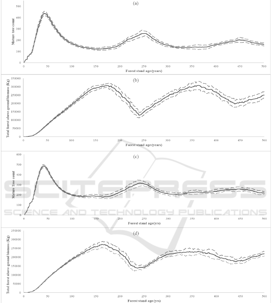
Figure 7: Trends in the development of the mangrove forest stand as it ages. Solid lines indicate the mean while the dashed
lines indicate the values a standard deviation away from the mean (a) Annual mature tree count at Site 2; (b) Annual total
forest AGB at Site 2; (c) Annual mature tree count at Site 3; (d) Annual total forest AGB at Site 3.
Sonneratia alba were second to dominate. At
salinity values greater than 30 ppt, only Avicennia
officinalis and Camptostemon philippinense have
significant dominance in the forest.
It is worth noticing that the dominance of mangrove
species changes drastically at around 25 ppt and 30
ppt as these values are the set upper boundaries for
optimum growth for low and mid salinity tolerant
SIMULTECH 2019 - 9th International Conference on Simulation and Modeling Methodologies, Technologies and Applications
162
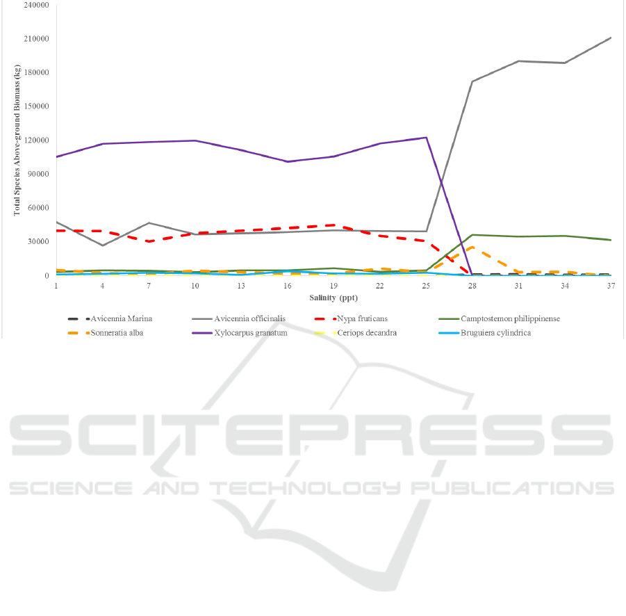
Figure 8: Dominance of eight species in KII Eco-park given different salinity conditions. Note that values of the above-ground
biomass between the shown salinity values in the x-axis are interpolations, hence are approximations of simulation results for
respective salinity values.
species, respectively. It is expected that adjusting
these values will drastically change the species
dominance curves.
Shading tolerance of each species also play a
significant role in the dominance curves of the
species. In the lower salinity values, Xylocarpus
granatum dominated over the other species even if it
is a low salt tolerant species. Given that the salinity
conditions do not hinder the growth of the species, the
shading tolerance played a vital role as Xylocarpus
granatum can still compete with other species even in
under-canopy conditions.
Lastly, the growth rates of species also play a role
in the dominance curves. Avicennia marina, Ceriops
decandra, and Bruguiera cylindrica may not be able
to dominate in the forest due to a combination of
either low salt and shade tolerance and low growth
rates
To summarize, three factors affect the dominance
curves of mangrove species: salt tolerance, shading
tolerance, and the growth rate. Because of these
factors, dominance curves of each species may
increase and decrease through a salinity gradient. At
some salinity range, a species may be more
dominating as some other species may grow slow,
hence it is the opportunity of the species to dominate.
7 CONCLUSION
This paper developed a model for simulating
mangrove forest stand dynamics. The model
simulates the development of mixed mangrove
forests on a 50 m x 50 m plot given the different
specific properties of each mangrove species and a set
salinity condition in the site.
Results of the model simulations given the salinity
conditions in a study site showed six of eight species
matched actual dominance level in the site. Model
simulations also displayed mangrove forest dynamics
such as gap dynamics and biomass dynamics. Lastly,
simulations showed the varying dominance of
different mangrove species given different salinity
conditions.
Given these results, the developed model is ready
to be used for different applications. The model may
be used for planning mangrove reforestation
programs, specifically to determine if species that
will be planted will be abundant given the site
conditions. The model can also be used in explaining
species zonation in a mangrove forest. Incorporation
of more environmental factors such as inundation
frequency, temperature, and biotic factors may better
explain observed distribution of mangrove species in
a forest. The model can also be restructured to
A Species-specific Individual-based Simulation Model of Mixed Mangrove Forest Stands
163

accommodate input so that it can be used for more
applications (e.g., using sea level rise data as input to
assess the effect of sea level rise to the distribution of
mangrove species).
ACKNOWLEDGEMENTS
This study is an extension of the works done by the
GeoSiMAS project of IAMBlueCECAM program.
REFERENCES
Berger, U. and Hildenbrandt, H., 2000. A new approach to
spatially explicit modelling of forest dynamics:
spacing, ageing and neighbourhood competition of
mangrove trees. Ecol. Model, 132, pp. 287–302.
Bojo, O., 1995. Sonneratiaceae. In: Soepadmo, E. and
Wong, K.M. (Eds.), Tree Flora of Sabah and Sarawak.
Ampang Press Sdn. Bhd., Kuala Lumpur, pp. 443-451.
Bormann, F.H. and Likens, G.E., 1979. Pattern and process
in a forested ecosystem. Springer-Verlag, New York,
pp. 253.
Botkin, D.B., Janaj, J.F., Wallis, J.R., 1972. Some
ecological consequences of a computer model of forest
growth. J. Ecol, 60, pp. 849-872.
CABI, 2018, Nypa fruticans (nipa palm), viewed 21
January 2019, <https://www.cabi.org/isc/datasheet/
36772>.
Chen, R. and Twilley, R.R., 1998. A gap dynamic model of
mangrove forest development along gradients of soil
salinity and nutrient resources. J. Ecol, 86, pp. 37–51.
Dangremond, E., Feller, I., Sousa, W., 2015. Environmental
tolerances of rare and common mangroves along light
and salinity gradients. Oecologia, 179(4), pp. 1187–
1198.
Duke, N., Ball, M., Ellison, J., 1998. Factors Influencing
Biodiversity and Distributional Gradients in
Mangroves. Global Ecology and Biogeography, 7, pp.
27-47.
FAO Ecocrop, 2018, Plant Search Form, viewed 21 January
2019, <http://ecocrop.fao.org/ecocrop/srv/en/
cropFindForm>.
Garcia, K., Gevaña, D., Malabrigo, P., 2013. Philippines'
Mangrove Ecosystem: Status, Threats, and
Conservation. Mangrove Ecosystems of Asia: Status,
Challenges and Management Strategies, pp. 81-94.
Giesen, W., Wulffraat, S., Zieren, M., 2007. Mangrove
Guidebook for Southeast Asia. FAO Regional Office
for Asia and the Pacific.
Grueters, U., Seltmann, T., Schmidt, H., Horn, H.,
Pranchai, A., Vovides, A.G., Peters, R., Vogt, J.,
Dahdouh-Guebas, F., Berger, U., 2014. The mangrove
forest dynamics model mesoFON. Ecol. Model, 291,
pp. 28–41.
Jiang J., DeAngelis D., Smith III T., Teh S., Koh H-L.,
2012. Spatial pattern formation of coastal vegetation in
response to external gradients and positive feedbacks
affecting soil porewater salinity: a model study.
Landscape Ecology, 27(1), pp. 109–119.
Keeton, W., Whitman, A., Mcgee, G., Goodale, C., 2011.
Late-Successional Biomass Development in Northern
Hardwood-Conifer Forests of the Northeastern United
States. Forest Science, 57, pp. 489-505.
Komiyama A., Ong J.E., Poungparn S., 2008. Allometry,
biomass, and productivity of mangrove forests: A
review. Aquatic Botany, 89(1), pp. 128-137.
Ma, R-Y., Zhang, J-L., Cavaleri, M., Sterck, F., Strijk, J.,
Cao, K-F., 2015. Convergent Evolution towards High
Net Carbon Gain Efficiency Contributes to the Shade
Tolerance of Palms (Arecaceae). PLOS ONE, 10(10).
Madani, L. and Wong, K.M., 1995. Rhizophoraceae. In:
Soepadmo, E. and Wong, K.M. (Eds.), Tree Flora of
Sabah and Sarawak. Ampang Press Sdn. Bhd., Kuala
Lumpur, pp. 321-349.
Reef, R. and Lovelock, C., 2015. Regulation of water
balance in mangroves. Annals of Botany, 115, pp. 385-
395.
Smith, T., 1992. Forest structure. In: Robertson, A.I. and
Alongi, D.M. (Eds.), Tropical mangrove ecosystems.
American Geophysical Union, Washington, D.C., pp.
101-136.
World Agroforestry, n.d. Wood Density. viewed 21 January
2019, <http://db.worldagroforestry.org/wd>.
SIMULTECH 2019 - 9th International Conference on Simulation and Modeling Methodologies, Technologies and Applications
164
