Neuroevolution with CMA-ES for Real-time Gain Tuning of a Car-like

Robot Controller

Ashley Hill

, Eric Lucet

and Roland Lenain

CEA, LIST, Interactive Robotics Laboratory, Gif-sur-Yvette, F-91191, France

Universit

e Clermont Auvergne, Irstea, UR TSCF, Centre de Clermont-Ferrand, F-63178 Aubi

ere, France

Keywords:

Neuroevolution, Machine Learning, Neural Network, Evolution Strategies, Gradient-free Optimization,

Robotics, Mobile Robot, Control Theory, Gain Tuning, Adaptive Control.

Abstract:

This paper proposes a method for dynamically varying the gains of a mobile robot controller that takes into

account, not only errors to the reference trajectory but also the uncertainty in the localisation. To do this,

the covariance matrix of a state observer is used to indicate the precision of the perception. CMA-ES, an

evolutionary algorithm is used to train a neural network that is capable of adapting the robot’s behaviour in

real-time. Using a car-like vehicle model in simulation. Promising results show signiﬁcant trajectory follow-

ing performances improvements thanks to control gains ﬂuctuations by using this new method. Simulations

demonstrate the capability of the system to control the robot in complex environments, in which classical static

controllers could not guarantee a stable behaviour.

1 INTRODUCTION

Mobile robots are used to accomplish different mis-

sions, their sensors being used to correctly and ef-

ﬁciently understand the robot’s environment. Those

sensors have varying degrees of certainty in their mea-

surement depending on the environment and their

properties. This limits the efﬁciency of robots us-

ing static controllers, as the tuning of their parame-

ters takes into consideration the nominal behaviour of

the robot, which has a negative effect on the robot’s

efﬁciency when operating in sub-nominal states. The

purpose of tuning these controllers is also to guaran-

tee a higher level of margins, which has a negative ef-

fect on robot performance during nominal states. This

compromise reduces the overall performance of the

robot. In control theory, noise robustness is an es-

sential quality (Ghorbel et al., 1991); it is therefore

relevant to use the noise information directly to adjust

control parameters in real-time.

In the ﬁeld of mobile robotics, ﬁnding an opti-

mal control policy is a challenging task. Especially in

complex environments where sensor precision varies

considerably and as so the level of noise in the system.

The aim of this paper is to integrate the noise into the

control policy in order to adjust the robot’s behaviour

to its complex environment. Different types of con-

trollers can be proposed (Jalali and Ghafarian, 2009;

Jiang et al., 2008; Doicin et al., 2016). However, tun-

ing controller gains relies on many parameters (Da-

ful, 2018). As a solution to the tuning problem, Neu-

ral networks have been used, with promising results

(Guo et al., 2009; Shu et al., 2015; Carlucho et al.,

2017); however such methods use small neural net-

works that are not capable of complex inference, and

are using the error or state vector as the basis for the

gradient which can cause instability if noisy.

CMA-ES

Controller

EKF

Robot

State

Measures

Control inputErrors

Setpoints

Errors, state

covariance,

curvature

Objective

function

Parameters

Gains

Figure 1: Control bloc diagram of the proposed method.

In green is the CMA-ES training method and in blue the

control loop with the neural network (NN).

In this paper, a new strategy for on-line gains

adaptation is propose and summarised in Figure 1.

CMA-ES (Hansen, 2016) is the optimisation algo-

rithm for the parameters of the neural network. The

neural network block takes parameters and environ-

mental information as inputs, and outputs the gains of

the controller. The controller uses the gains deﬁned

by the neural network in order to effectively follow

Hill, A., Lucet, E. and Lenain, R.

Neuroevolution with CMA-ES for Real-time Gain Tuning of a Car-like Robot Controller.

DOI: 10.5220/0007927103110319

In Proceedings of the 16th International Conference on Informatics in Control, Automation and Robotics (ICINCO 2019), pages 311-319

ISBN: 978-989-758-380-3

311

the requested trajectory. The robot’s dynamics sim-

ulate the behaviour of the robot. The noise mimics

real world conditions, and so an extended Kalman ﬁl-

ter (EKF) is used to observe the state of the robot. It

provides the estimated state ˆx and the corresponding

covariance matrix P.

In the following, the paper is structured into three

main sections before conclusions. The second sec-

tion presents all the localisation, modelling, and con-

trol algorithms applied to the robot. The third section

is dedicated to the presentation of gains adaptation.

Finally, results are detailed and discussed along with

perspectives.

2 LOCALISATION PROCESS AND

CONTROL

2.1 Modelling

The focus of this study is to adapt the control policy of

a car-like mobile robot to the precision of the percep-

tion, the lateral error, the angular error, and the current

curvature of the trajectory; using a neuroevolution al-

gorithm. In order to train the system and test it, a

model of the robot was used to simulate its behaviour.

The model is fairly representative of the task and had

been used in previous works (Jaulin, 2015). The robot

is described by the following kinematic model:

X =







˙x

˙y

˙v













v cos(θ) +α

v sin(θ) + α

tan(u

+α

)

+ α







(1)

The state variables are: x,y the coordinates of the

robot in the world frame, θ its heading, L its wheel-

base, and v its rear velocity. u

and u

are the acceler-

ation and steering inputs respectively. α

is the white

Gaussian noise of the i state variable.

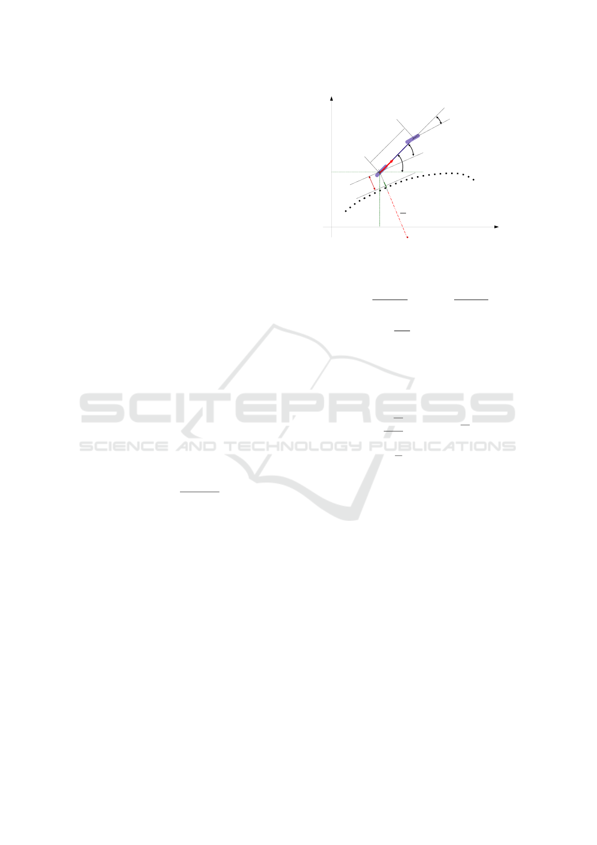
In Figure 2, u

is the steering angle of the robot

(Ackermann angle) and constitutes the control input,

is the distance from the robot to the path, ψ is the

robot heading, (D) is the trajectory, κ is the curvature

of the trajectory, L is the wheelbase of the robot. The

angular deviation ε

is representative of the difference

between the robot heading and the orientation of the

trajectory.

2.2 Control Law

The robot has to complete a task, which is in our case

following a trajectory. To accomplish this, the follow-

(D)

Figure 2: The mobile robot studied.

ing controller is used:

= arctan



L cos



) +

cos

(ε

)



(2)

with e

= tanε

−





is the relative orientation

error of the robot to reach its trajectory (i.e. ensur-

ing the convergence of ε

to 0). This control detailed

in (Lenain et al., 2017) guaranties the stabilisation of

the robot to its reference trajectory, providing a rele-

vant choice for the gains k

and k

. Theoretically, a

relevant choice for these gains may be:

and k

= 2

it implies k

× k

and guaranties that the con-

straint k

> k

is respected, we then get our ﬁnal con-

troller with k

the controller gain. As a result, the

control law (2) has only one parameter k

, deﬁning

the theoretical distance of convergence of the robot to

the trajectory (as it has been proven in (Lenain et al.,

2017)). As a result, the higher the gain is, the more

reactive the robot is. However the sensor noise as well

as delays in the low level may lead to instability. The

choice of this gain has to then be made with respect

to localisation properties.

2.3 Robot Localisation

In order to feed the control law (2) with lateral and

angular error, the state vector deﬁned by (1) has to be

known. For estimating the state of the robot, an EKF

is proposed. It assists in determining the linear speed,

the x, y position, and the heading. It is widely used

due to its simplicity and robustness.

In the proposed system, P is the covariance matri-

ces of the estimation and it is used to determine the

level of precision of the perception. A novelty of this

paper is that both the estimate and the corresponding

ICINCO 2019 - 16th International Conference on Informatics in Control, Automation and Robotics

312

covariance matrix are integrated in the tuning of the

Controller. The observed variables are used to control

the robot along a path. Even though the controller is

easy to implement, the tuning of its parameters is not

a simple task and is a large research area (Ho et al.,

1996; Tyreus and Luyben, 1992; Hang et al., 2002).

3 CONTROL GAINS

ADAPTATION

The nature of the environment forces the mobile

robot’s perception to vary in precision. These changes

in precision will be given by the changes in the co-

variance matrix of the EKF. Therefore, the controller

gains must adjust periodically. In order to adapt the

controller’s parameters to the level of precision in the

perception, but also to the properties of the trajectory,

a neural network is used. The network will tune the

controller in real-time, based on the tracking errors,

the path curvature and the covariance matrix of the

EKF.

3.1 The Neural Network Model

Hidden layer

100

Hidden layer

Input layer

Output layer

Figure 3: Graphical representation of the used neural net-

work. With 7 neurons in the input layer, 3 hidden layers of

40, 100, and 10 neurons respectively, and 1 neuron for the

output layer. all the layers except the output layer go though

a hyperbolic tangent function as the activation function.

Neural networks (NN) are highly connected systems

which are used to model complex non-linear func-

tions. In neural networks the inputs are transformed

through matrix multiplications and non-linear activa-

tion functions, in order to obtain a universal function

estimator through the tuning of the weights (Hornik

et al., 1990). The used neural network (see Figure 3)

has as input the vector of concatenated values for: the

lateral error ε

, the angular error ε

, the curvature of

the trajectory κ, and the diagonal of the EKF covari-

ance matrix P. As output, this neural network returns

a vector corresponding to each controller gain respec-

tively. The training of the neural network is the pro-

posed neuroevolution algorithm, which means that an

evolution strategy will be used to optimise the neural

network. Evolution strategies are stochastic optimi-

sation algorithms (Beyer and Schwefel, 2002). The

great advantage of this family of algorithms is that

they do not need to calculate any gradient when opti-

mising a neural network. This allows to reduce com-

putation when training and it is robust to noisy re-

turn signals (e.g. reward, objective function, etc ...)

unlike reinforcement learning for example (Salimans

et al., 2017). All evolutionary algorithms go through

the same steps: mutation, evaluation, selection, repro-

duction and repeat until a termination criterion is met.

There exists multiple algorithms in the family of evo-

lution strategies, a few of them were considered, es-

pecially genetic algorithms. However, the CMA-ES

(Hansen, 2016) optimisation algorithm has shown its

superiority in highly modal, non-convex, noisy func-

tions (Hansen et al., 2010); such as the highly non-

convex search spaces of neural networks with a noisy

objective function (Salimans et al., 2017; Risi and To-

gelius, 2014; Such et al., 2017).

3.2 CMA-ES Neuroevolution

To adjust the behaviour of the robot, a neural net-

work was chosen to adjust the parameters of the con-

troller. This neural network’s architecture was chosen

based on previous work and experimentation, in or-

der to be able to infer a complex enough non linear

outputs from the given inputs. Neural network pa-

rameters, such as weights and biases, are optimised

by the CMA-ES method during the ofﬂine training

phase. The CMA-ES optimisation algorithm starts by

generating an initial population of parameters for the

neural network, by drawing samples from the follow-

ing distribution:

g+1

∼ m

+ σ

N (0,C

) f or k = 1, ..., λ (3)

with m

the mean vector of the current generation, σ

the step size vector of the generation, C

the covari-

ance matrix of the generation which differs from the

covariance matrix of the Kalman ﬁlter, and λ the size

of the population. CMA-ES uses the covariance ma-

trix to chose the optimal direction of the search and

the step size over every parameter to know the op-

timal length of the step to take between consecutive

generations. Here both phases are presented. The ﬁrst

one is the training phase where the neural network is

optimised to learn the behaviour which robot is in-

tended to have. After this, the neural network and the

controller are deployed into the robot to work online.

Neuroevolution with CMA-ES for Real-time Gain Tuning of a Car-like Robot Controller

313

During the online training phase, a simulation of the

robot’s kinematics is used to simulate its behaviour,

and a controller is used to follow the requested path.

The robot’s state is measured by adding noise to the

simulated state, and an EKF is then used to observe

the state of the robot. Once the online training is

completed and the objective function is calculated, the

CMA-ES method then optimises the neural network

parameters based on the objective function.

The CMA-ES generates a population of neural

networks based on the architecture. Each neural net-

work is used by the simulation to generate controller

gains for each timestep using the current errors, cur-

vature, and EKF covariance matrix. These parameters

are then used to control the robot. For each neural

network, a series of simulated trajectories are used in

order to calculate the objective function of the neural

network using the robot over many examples to avoid

overﬁtting; this objective function is the criterion for

comparing the performance of each neural network.

CMA-ES puts the neural networks found in order,

based on their score. A set of the best preforming

individuals are then used to produce the next genera-

tion and the cycle continues until a stopping criterion

is met. By the end of the training, the resulting neu-

ral network is the one with the lowest score. For a

neural network to have the best score, it must adapt

the behaviour of the robot so as to decrease the er-

ror by considering the real state and not the observed

one. For this to happen, the neural network has to

choose high gains on the controller to force the robot

to follow the reference, especially when cornering or

correcting any lateral errors. However, when the level

of noise is high, it must lower the mean values of the

gains to not have an oscillatory behaviour which com-

promises both the mechanical structure of the robot

and the comfort of the passengers in the case of occu-

pied vehicles.

For the deployment phase, the trained neural net-

work and the controller are deployed into the robot.

The neural network does not consume too much re-

source as it is only used for inference of the controller

gains and not for training.

3.3 The Objective Function

The objective function is an essential part of evolution

strategies, it is what the algorithm tries to minimise in

order to ﬁnd the best local optimum for the search

space. To minimise the objective function, CMA-ES

tweaks the parameters of the neural network in order

to have the lowest possible value; this tweaking of

the parameters is what is called learning, because the

model is in fact a system that has the capacity to learn

certain behaviours, and is adapting to reach said be-

haviours. Since the objective function determines the

behaviour of the neural networks, we have tested the

following objective functions formulated as:

∑

τ=0

|ε

(τ)| + |ε

(τ)L| (4)

∑

τ=0

|ε

(τ)| + |ε

(τ)L| + |u

(τ)L| (5)

∑

τ=0

|ε

(τ)| + |ε

(τ)L| + k

steer

(τ)L| (6)

with ε

the lateral error, ε

the angular error, u

the

steering input, L the wheelbase of the robot, k

steer

the

weight of the steering input in the objective function,

and T the total timesteps of the simulation. The abso-

lute value of the errors and steering input are used as

we are measuring the accumulated amplitude of these

values. Since the objective functions takes into ac-

count both the lateral and the angular errors, using

the accumulation of them at the end of the simulations

guarantees a coherent objective function that will per-

form a similar trade off as the controller, meaning it

wont degrade the overall performance in order to op-

timise one of the errors.

4 RESULTS AND DISCUSSIONS

Here are presented the results of the developed sys-

tem. Since evolution strategies are comparable to re-

inforcement learning methods (Salimans et al., 2017),

we will compare this method to reinforcement learn-

ing methods using the negative amplitude of lateral

and angular errors as its rewards, and a constant gain

method trained using CMA-ES on the same objective

function as the proposed method, similarly to existing

methods (Wakasa et al., 2010; Sivananaithaperumal

and Baskar, 2014; Marova, 2016). Tests are focused

on the trained system and not on the training phase.

This section is divided into two main parts. In the

ﬁrst part: The experimental environment is presented.

Then, the limitations of using a constant gain method

are shown qualitatively. Then, the qualitative results

from the training phase are presented. Finally, the

system performance is compared to results in same

conditions with a ﬁx gain controller and with a rein-

forcement learning algorithm. And in the second part,

the results are discussed in a general context and im-

provements are suggested.

ICINCO 2019 - 16th International Conference on Informatics in Control, Automation and Robotics

314

4.1 Results

4.1.1 Simulated Environment

The training setup for all the methods were on a sim-

ulated robotic environment, with a cinematic model,

without wheel slipping, and without control latency,

written in Python and C, where the robot must follow

a series of trajectories, with noisy position measure-

ments distributed randomly in zones along the trajec-

tories to simulated GPS-like perturbations, and with

a randomly placed change lane along the trajectories

to simulated abrupt changes in the setpoints. This al-

lows rather realistic types of noises that a robot can

encounter that will cause instability and higher over-

all errors to occurs. The trajectories are: a line, a sine

wave, a parabola, a Bezier spline in an sigmoid shape

called spline1, and a Bezier spline in a u-turn shape

called spline2. With the perturbations and trajecto-

ries, this setup helps prevent CMA-ES or reinforce-

ment learning methods from falling into bad local op-

timums and overﬁtting, due to the high randomness of

the perturbations and the variations in the trajectories.

4.1.2 Limitations of the Constant Gain Model

An ideal gain model must allow the controller asso-

ciated to the gains, to simultaneously minimise the

errors and not be too reactive to noise present in said

error. In our case study this means ﬁnding the gains

that are able to follow a line as closely as possible,

whilst avoiding undesirable reactions to noise that can

induce unstable behaviours.

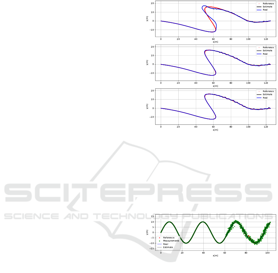
Looking at ﬁgure 4, we can see the compromise

a constant gain model must achieve. In the ﬁrst plot

with a small gain, we can see the robot having trouble

following the line when the corners occur; however

it is quite steady and stable in the noisy region of the

trajectory. In the third plot with the very high gain, we

see the complete opposite of this, the robot becomes

completely unstable in the perturbed region; however

it was very close to the curve in the high accuracy

region. And in the second plot with a gain that is mid-

way of the ﬁrst and third plot, we can see some dif-

ﬁculties following the lines in the stable region, and

some instability and oscillation in the noisy region.

One can then see the limitations of a constant gain

model that must reach a paradoxical compromise be-

tween contradicting gains. In this case, the clear solu-

tion is an adaptive model, such as the proposed con-

tribution.

Figure 4: The x,y view of the simulation using the spline1

trajectory and a constant gain model. Midway through the

trajectory noise is applied to the position measurements.

Above: The ﬁrst plot with a low gain of 0.1. Middle: The

second plot with a high gain of 3.0. Below: The third plot

with a very high gain of 7.0.

4.1.3 Qualitative Results

In order to help visualise the gain adaptation to the

perturbations, the trajectory in ﬁgure 5 is used in the

following results:

Figure 5: The x,y view of the simulation using the sine tra-

jectory. Midway through the trajectory noise is applied to

the position measurements, and then a change lane occurs

just before the last corner.

After training, (see Figure 6), the real vehicle han-

dles the EKF covariance matrix’s errors, the curvature

of the trajectory, and even the lateral error due to a

change lane.

It can be seen that, as expected, a higher gain is

computed when cornering, when an unexpected per-

turbation occurs, and when the position accuracy is

high. In contrast, the gain is reduced when the posi-

tion accuracy is too low, in order to avoid a possibly

unstable behaviour.

Furthermore, when using objective functions ob

and ob

, the neural network is able to lower signif-

icantly the oscillatory behaviour of the steering, as

shown in Figure 7.

Neuroevolution with CMA-ES for Real-time Gain Tuning of a Car-like Robot Controller

315

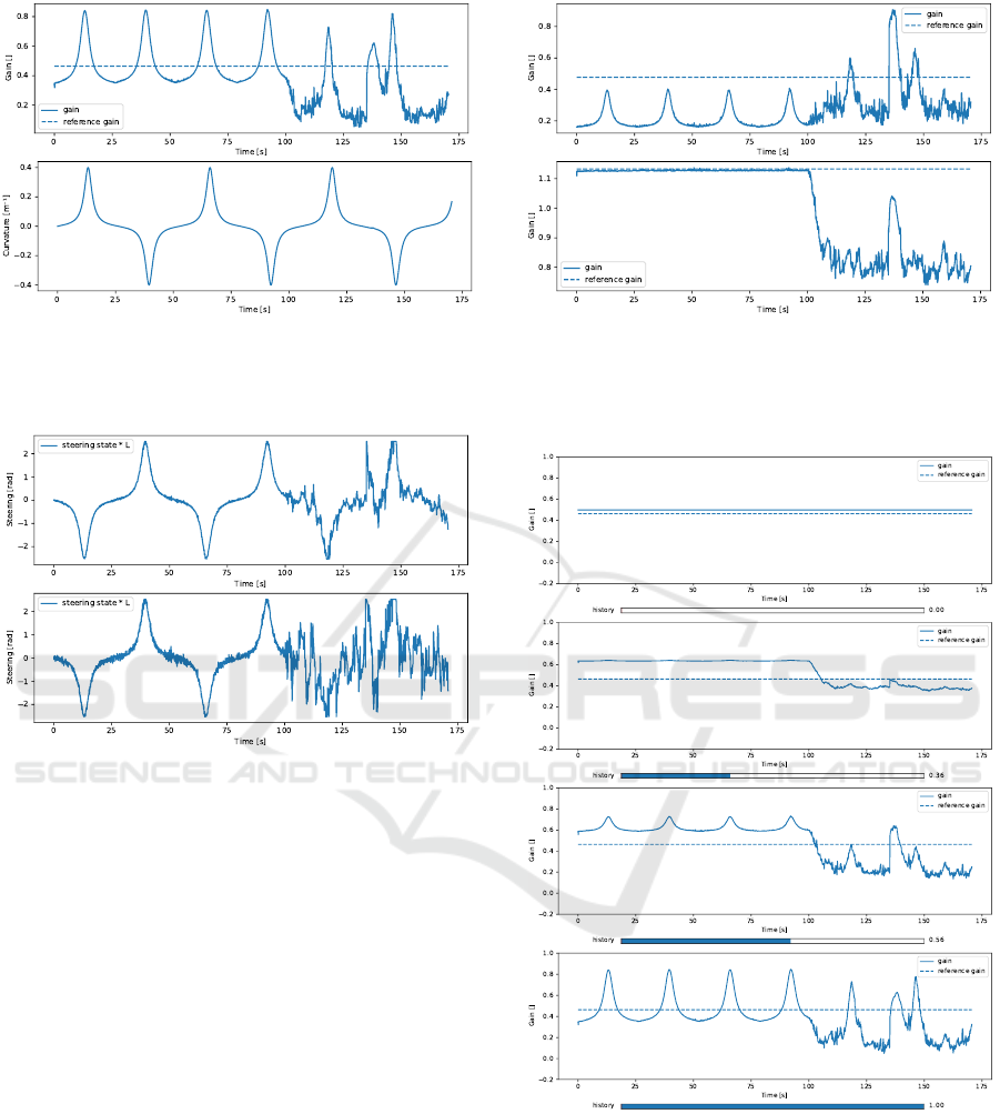
Figure 6: Above: the gain outputed by the neural network

in the solid line, and the chosen constant gain value in the

dashed line. Below: the curvature of the trajectory over

time.

Figure 7: Steering input u

over time by using the proposed

method. Above: when trained with the objective function

. Below: when trained with the objective function ob

Additional experiments such as ablation over the

given inputs to the neural network were done. The

EKF covariance matrix seems to be an invaluable in-

formation for predicting a useful gain, as when trained

without it causes a much lower gain overall, as it can-

not know the regions where instability occurs (see

Figure 8). Also the curvature is helping to obtain a

lower objective function overall when the trajectory

is not curved, allowing for smoother control.

Some tools were developed in order to understand

the training process in further details. On the history

of the trained network displayed in Figure 9, we can

see that the CMA-ES method ﬁrst optimises the gain

using the covariance of the Kalman ﬁlter, then using

the lateral error, and then using the curvature. This

order makes sense, as it is from the most to the least

impactful to the objective function through the gain,

and as such, it should be optimised in this order.

Figure 8: The gain outputed by the neural network in the

solid line, and the optimal constant gain value in the dashed

line. Above: when trained without using the EKF covari-

ance matrix as input. Below: when trained without using

the curvature of the trajectory as input.

Figure 9: Gain values over the training generations. The

gain outputed by the neural network in the solid line, and

the optimal constant gain value in the dashed line.

4.1.4 Quantitative Results

In order to help verify quantitatively the relevance of

our results, we used the Welch t-test (Welch, 1947)

over the distribution of the values of the objective

functions, with the null hypothesis being that our

method produces the same results as the constant gain

ICINCO 2019 - 16th International Conference on Informatics in Control, Automation and Robotics

316

method. The resulting test returns p-values, that are

the probability of obtaining these results if the null

hypothesis is true; as such, if the p-value is lower than

1.00e

−2

we can consider the null hypothesis being re-

jected, and show the signiﬁcance of our results.

We used two methods to compare our results

quantitatively. The ﬁrst is to see the improvement

relative to a static gain controller using the objective

function with a Welch t-test over multiple trajectories

and seeds. The second is to see the improvement rel-

ative to a gain tuned by reinforcement learning meth-

ods using the objective function with over multiple

trajectories and seeds. These two methods should al-

low us to see how the suggested method improves the

quality of the control over the traditional constant gain

method and over reinforcement learning based meth-

ods.

Table 1: Welch test p-values between ﬁxed gain and the

suggested method, for every trajectory over the objective

functions. With k

steer

= 0.5.

trajectory ob

line 3.22e−2 1.80e−8 7.01e−5

sine 1.61e−4 4.07e−9 6.06e−7

parabola 6.53e−12 4.20e−21 1.49e−17

spline1 2.09e−28 3.63e−21 5.08e−19

spline2 3.48e−1 8.42e−16 1.49e−9

We can see from the table 2 that across all the

objective functions and the trajectories, that the

proposed method obtained between 3% to 20%

improvement with an average of 10% improvement

over the constant gain method. Furthermore, with the

table 1 we can see that the p-values associated with

these improvements, are for the most part signiﬁcant,

except for the line and spline2 trajectories, which

are both hard to improve upon as the ﬁrst is a very

easy trajectory for the constant gain, and the second

is quite hard for the robot model to follow with its

given design. Nevertheless, the other results are quite

signiﬁcant and do indeed show the beneﬁt of this

method when compared to the constant gain method.

As discussed earlier, CMA-ES based neuroevolu-

tion can obtain similar if not better performance when

compared to reinforcement learning (RL) based meth-

ods. The trade-off is that neuroevolution is more sta-

ble to noise, but requires more time to train than rein-

forcement learning. Here four commonly used mod-

els where tested on the training environment: Soft ac-

tor critic (labeled SAC) (Haarnoja et al., 2018), Prox-

imal policy optimization (labeled PPO) (Schulman

et al., 2017), Deep deterministic policy gradient (la-

beled DDPG) (Lillicrap et al., 2015), and Advantage

actor critic (labeled A2C) (Mnih et al., 2016); using

the RL library stable-baselines (Hill et al., 2018).

We can see from the table 3 that none of the reinforce-

ment learning models where capable of reaching even

the baseline constant gain model; with most of the

models between 19% and 3870% with an average of

588% of degradation in performance when compared

to the constant gain model. Considering the scale of

the amplitude and variance of the performance loss,

no t-test was performed on this dataset.

4.2 Discussion

Neuroevolution is used to tune controller gains in

real-time after a training phase. As mentioned before,

the CMA-ES optimises a neural network, then the

said neural network tunes the controller gains. The

proposed controller was used due to its simplicity and

ease of use. The objective was to develop an adapt-

able system that works with different types of con-

trollers whose parameters must be tuned.

As demonstrated in the results section, the pro-

posed method outperforms the traditional constant

gain method by a signiﬁcant amount; as it is capable

of adapting the robot behaviour to the environment

using the information present in the control loop. It is

able to achieve such performance by minimising the

wanted objective function through the CMA-ES train-

ing.

We also showed that modern reinforcement learn-

ing methods are not capable of learning a beneﬁcial

behaviour in the same environment. This is probably

due to the fact that the reward signal depends on the

information in the control loop, such as lateral and an-

gular errors; as in our experiments, they become very

noisy due to the position noise. This noise on the re-

ward signal prevents the critic of actor critic models

from correctly converging, causing erratic learning.

This ﬂaw does not occurs when using CMA-ES, as

it is inherently resilient to noisy objective functions

(Hansen, 2016; Salimans et al., 2017).

It is important to note that the selection of the ob-

jective function is very important to the quality of

the gain tuning, as the optimisation can compromise

the performance of other features. For example dur-

ing experimentation, the objective function ob

had

higher lateral error when compared to ob

, however

this is a trade off as ob

is more stable with respect to

the steering.

The training time for the method was about 5

hours wall time using 8 CPU cores, and can be scaled

extremely well with more CPUs thanks to the CMA-

ES method (Salimans et al., 2017). This training is

only feasible in simulation however, as the 5 hours of

training time is the equivalent of 1 simulated year. To

Neuroevolution with CMA-ES for Real-time Gain Tuning of a Car-like Robot Controller

317

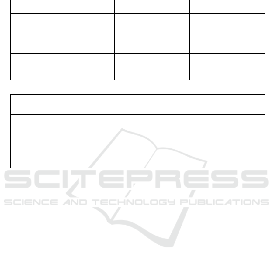
Table 2: The values of the objective functions for every trajectory. With k

steer

= 0.5.

trajectory CMA-ES NN ﬁxed gain CMA-ES NN ﬁxed gain CMA-ES NN ﬁxed gain

line 27.41

(±1.98)

28.30

(±2.08)

41.60

(±2.34)

48.20

(±2.45)

36.63

(±2.63)

40.46

(±4.65)

sine 39.81

(±2.18)

41.54

(±2.18)

144.76

(±2.86)

151.70

(±2.83)

94.11

(±2.32)

98.66

(±2.37)

parabola 64.41

(±2.90)

69.10

(±3.04)

98.73

(±3.39)

125.29

(±4.02)

83.38

(±3.27)

101.62

(±4.00)

spline1 52.34

(±2.14)

59.79

(±2.52)

117.66

(±3.04)

142.04

(±3.45)

87.30

(±3.07)

105.43

(±3.54)

spline2 68.33

(±2.59)

71.76

(±25.26)

147.32

(±3.18)

164.94

(±4.45)

110.03

(±3.12)

119.04

(±3.79)

Table 3: The values of the objective function ob

for every trajectory with RL methods.

trajectory CMA-ES NN SAC PPO DDPG A2C ﬁxed gain

line 41.60

(±2.34)

60.99

(±22.21)

115.11

(±57.10)

158.14

(±4.09)

57.52

(±15.12)

48.20

(±2.45)

sine 144.76

(±2.86)

1140.52

(±3004.65)

2403.93

(±2824.32)

309.18

(±5.79)

280.51

(±175.61)

151.70

(±2.83)

parabola 98.73

(±3.39)

191.48

(±2.43)

389.65

(±6.34)

417.99

(±6.23)

208.80

(±26.57)

125.29

(±4.02)

spline1 117.66

(±3.04)

508.24

(±152.24)

2864.41

(±14.31)

272.20

(±5.27)

542.85

(±4.47)

142.04

(±3.45)

spline2 147.32

(±3.18)

6563.63

(±3310.81)

3169.80

(±23.61)

258.85

(±26.39)

437.22

(±736.97)

164.94

(±4.45)

address the simulation issue, transfer learning could

be used to bridge the difference between simulated

and real world robotics. For example using domain

randomisation (OpenAI et al., 2018; Tan et al., 2018),

or by learning the gap between the simulation and the

real world (Golemo et al., 2018).

Further care should be taken should this method

be used in the real world, as even though the p-

values and objective functions values are favourable,

the method can have unexpected behaviour because

it is not currently possible to prove the stability of

method due to neural networks being black boxes and

CMA-ES not having a proof of convergence; this can

be mitigated with a supervisor that can replace the

method with a constant gain in unseen states, or by

clipping gain between certain bounds.

5 CONCLUSIONS

This paper presents a method of neuroevolution,

which is used to train a neural network to then tune

a controller in real time in order to adapt a robot’s

behaviour to a varying level of precision in the per-

ception. The proposed method has been shown to im-

prove the overall performance in the context of mo-

bile robotics when compared with constant gain mod-

els or reinforcement learning methods. Furthermore,

the proposed method can be used with varying con-

trollers in many different applications, such as nav-

igation in urban landscapes, agricultural application,

or even drones. Many possible variants exist of this

method that could be put in application, such as vari-

ants of the CMA-ES algorithm could be used, or even

the possible variants of the objective function for dif-

ferent tasks. In this paper, ﬁrst simulation tests have

been achieved to prove the theoretical validity of the

proposed approach, accounting for sensors noises and

low level settling times. Further experimentation with

existing adaptive control algorithms, and experimen-

tation with real world robots are required for future

works, especially with respect to grip conditions.

REFERENCES

Beyer, H.-G. and Schwefel, H.-P. (2002). Evolution

strategies–a comprehensive introduction. Natural

computing, 1(1):3–52.

Carlucho, I., Paula, M. D., Villar, S. A., and Acosta, G. G.

(2017). Incremental q-learning strategy for adaptive

pid control of mobile robots. Expert Systems with Ap-

plications, 80:183 – 199.

Daful, A. G. (2018). Comparative study of pid tuning meth-

ods for processes with large small delay times. In 2018

Advances in Science and Engineering Technology In-

ternational Conferences (ASET), pages 1–7.

ICINCO 2019 - 16th International Conference on Informatics in Control, Automation and Robotics

318

Doicin, B., Popescu, M., and Patrascioiu, C. (2016). Pid

controller optimal tuning. In 2016 8th International

Conference on Electronics, Computers and Artiﬁcial

Intelligence (ECAI), pages 1–4.

Ghorbel, F., Fitzmorris, A., and Spong, M. W. (1991). Ro-

bustness of adaptive control of robots: theory and ex-

periment. In Advanced Robot Control, pages 1–29.

Springer.

Golemo, F., Taiga, A. A., Courville, A., and Oudeyer, P.-Y.

(2018). Sim-to-real transfer with neural-augmented

robot simulation. In Billard, A., Dragan, A., Peters,

J., and Morimoto, J., editors, Proceedings of The 2nd

Conference on Robot Learning, volume 87 of Pro-

ceedings of Machine Learning Research, pages 817–

828. PMLR.

Guo, B., Liu, H., Luo, Z., and Chen, W. (2009). Adaptive

pid controller based on bp neural network. 2009 In-

ternational Joint Conference on Artiﬁcial Intelligence,

pages 148–150.

Haarnoja, T., Zhou, A., Abbeel, P., and Levine, S. (2018).

Soft actor-critic: Off-policy maximum entropy deep

reinforcement learning with a stochastic actor. CoRR,

abs/1801.01290.

Hang, C., Astrom, K., and Wang, Q. (2002). Relay feedback

auto-tuning of process controllers—a tutorial review.

Journal of process control, 12(1):143–162.

Hansen, N. (2016). The CMA evolution strategy: A tutorial.

CoRR, abs/1604.00772.

Hansen, N., Auger, A., Ros, R., Finck, S., and Po

ık, P.

(2010). Comparing results of 31 algorithms from

the black-box optimization benchmarking bbob-2009.

In Proceedings of the 12th Annual Conference Com-

panion on Genetic and Evolutionary Computation,

GECCO ’10, pages 1689–1696, New York, NY, USA.

ACM.

Hill, A., Rafﬁn, A., Ernestus, M., Traore, R., Dhariwal,

P., Hesse, C., Klimov, O., Nichol, A., Plappert, M.,

Radford, A., Schulman, J., Sidor, S., and Wu, Y.

(2018). Stable baselines. https://github.com/hill-a/

stable-baselines.

Ho, W. K., Gan, O., Tay, E. B., and Ang, E. (1996). Per-

formance and gain and phase margins of well-known

pid tuning formulas. IEEE Transactions on Control

Systems Technology, 4(4):473–477.

Hornik, K., Stinchcombe, M., and White, H. (1990). Uni-

versal approximation of an unknown mapping and

its derivatives using multilayer feedforward networks.

Neural Networks, 3(5):551 – 560.

Jalali, L. and Ghafarian, H. (2009). Maintenance of robot’s

equilibrium in a noisy environment with fuzzy con-

troller. In 2009 IEEE International Conference on

Intelligent Computing and Intelligent Systems, vol-

ume 2, pages 761–766.

Jaulin, L. (2015). Mobile Robotics. Mobile Robotics.

Jiang, L., Deng, M., and Inoue, A. (2008). Support vec-

tor machine-based two-wheeled mobile robot motion

control in a noisy environment. Proceedings of the In-

stitution of Mechanical Engineers, Part I: Journal of

Systems and Control Engineering, 222(7):733–743.

Lenain, R., Deremetz, M., Braconnier, J.-B., Thuilot, B.,

and Rousseau, V. (2017). Robust sideslip angles ob-

server for accurate off-road path tracking control. Ad-

vanced Robotics, 31(9):453–467.

Lillicrap, T. P., Hunt, J. J., Pritzel, A., Heess, N., Erez, T.,

Tassa, Y., Silver, D., and Wierstra, D. (2015). Contin-

uous control with deep reinforcement learning. CoRR,

abs/1509.02971.

Marova, K. (2016). Using CMA-ES for tuning coupled

PID controllers within models of combustion engines.

CoRR, abs/1609.06741.

Mnih, V., Badia, A. P., Mirza, M., Graves, A., Lillicrap,

T. P., Harley, T., Silver, D., and Kavukcuoglu, K.

(2016). Asynchronous methods for deep reinforce-

ment learning. CoRR, abs/1602.01783.

OpenAI, Andrychowicz, M., Baker, B., Chociej, M.,

ozefowicz, R., McGrew, B., Pachocki, J. W., Pa-

chocki, J., Petron, A., Plappert, M., Powell, G., Ray,

A., Schneider, J., Sidor, S., Tobin, J., Welinder, P.,

Weng, L., and Zaremba, W. (2018). Learning dexter-

ous in-hand manipulation. CoRR, abs/1808.00177.

Risi, S. and Togelius, J. (2014). Neuroevolution in

games: State of the art and open challenges. CoRR,

abs/1410.7326.

Salimans, T., Ho, J., Chen, X., Sidor, S., and Sutskever, I.

(2017). Evolution Strategies as a Scalable Alternative

to Reinforcement Learning. ArXiv e-prints.

Schulman, J., Wolski, F., Dhariwal, P., Radford, A., and

Klimov, O. (2017). Proximal policy optimization al-

gorithms. CoRR, abs/1707.06347.

Shu, H., Wang, X., and Huang, Z. (2015). Identiﬁcation

of multivariate system based on pid neural network.

In 2015 Sixth International Conference on Intelligent

Control and Information Processing (ICICIP), pages

199–202.

Sivananaithaperumal, S. and Baskar, S. (2014). Design

of multivariable fractional order pid controller us-

ing covariance matrix adaptation evolution strategy.

Archives of Control Sciences, 24(2):235–251.

Such, F. P., Madhavan, V., Conti, E., Lehman, J., Stanley,

K. O., and Clune, J. (2017). Deep neuroevolution: Ge-

netic algorithms are a competitive alternative for train-

ing deep neural networks for reinforcement learning.

CoRR, abs/1712.06567.

Tan, J., Zhang, T., Coumans, E., Iscen, A., Bai, Y., Hafner,

D., Bohez, S., and Vanhoucke, V. (2018). Sim-to-

real: Learning agile locomotion for quadruped robots.

CoRR, abs/1804.10332.

Tyreus, B. D. and Luyben, W. L. (1992). Tuning pi con-

trollers for integrator/dead time processes. Industrial

& Engineering Chemistry Research, 31(11):2625–

2628.

Wakasa, Y., Kanagawa, S., Tanaka, K., and Nishimura,

Y. (2010). PID Controller Tuning Based on the Co-

variance Matrix Adaptation Evolution Strategy. IEEJ

Transactions on Electronics, Information and Sys-

tems, 130:737–742.

Welch, B. L. (1947). The generalization of ‘student’s’ prob-

lem when several different population varlances are

involved. Biometrika, 34(1-2):28–35.

Neuroevolution with CMA-ES for Real-time Gain Tuning of a Car-like Robot Controller

319