Optimal Active Target Localisation Strategy with Range-only
Measurements
Shaoming He
a
, Hyo-Sang Shin
b
and Antonios Tsourdos
c
School of Aerospace, Transport and Manufacturing, Cranfield University, College Road, Cranfield, MK43 0AL, U.K.
Keywords: Target Localisation, Range-only Measurement, Optimal Manoeuvre.
Abstract:
This paper investigates the problem of one-step ahead optimal active sensing strategy to minimise estimation
errors with range-only measurements for non-manoeuvring target. The determinant of Fisher Information
Matrix (FIM) is utilized as the objective function in the proposed optimisation problem since it quantifies the
volume of uncertainty ellipsoid of any efficient estimator. In consideration of physical velocity and turning
rate constraints, the optimal heading angle command that maximises the cost function is derived analytically.
Simulations are conducted to validate the analytical findings.
1 INTRODUCTION
The past few years have witnessed an increasing inter-
est in the development and employment of small-scale
unmanned robots in both civil and military applica-
tions. One particular interesting mission of small-
scale unmanned robots is to track and localize targets
of interest in an automated fashion since reliable tar-
get tracking is a fundamental and key enabling tech-
nology in many practical applications, such as vehicle
navigation, situational awareness and public surveil-
lance (Atanasov et al., 2014; Salaris et al., 2017).
One main challenge for the operations of these small-
scale robots in target localisation is that they are typi-
cally constrained by limited payload, power and en-
durance. Therefore, only limited information, e.g.,
bearing-only or range-only, can be gathered due to the
limits of sensor availability.
It is well-known that the relative geometry be-
tween the observer and the target poses great effects
on the achievable localisation performance (Bishop
et al., 2010). For this reason, active sensing that finds
the optimal path or trajectory for information gain
maximisation can yield significant benefits to improv-
ing the perceptual results in target localisation (Bajcsy
et al., 2018). Through numerically maximising the
determinant of FIM over a finite horizon, optimal ob-
server trajectory for bearing measurements gathering
a
https://orcid.org/0000-0001-6432-5187
b
https://orcid.org/0000-0001-9938-0370
c
https://orcid.org/0000-0002-3966-7633
to localize a single target was proposed in Tokekar
et al. (2011). The rationale of leveraging FIM lies
in that it prescribes a lower bound of target localisa-
tion error covariance of any efficient estimation algo-
rithm (Taylor, 1979). Therefore, the determinant of
FIM can be utilized as a performance metric to quan-
tify the volume of the error uncertainty ellipsoid. Ex-
cept for FIM, the trace of error covariance, which di-
rectly quantifies the average estimation performance,
was also utilized to find the proper path for target
localisation using bearing-only measurements (Logo-
thetis et al., 1997; Zhou et al., 2011). Note that most
approaches utilize numerical methods to find the op-
timal solutions and consequently require high com-
putational burden. To alleviate the computational is-
sue, an analytical solution was proposed in (He et al.,
2019) using geometric analysis for bearing-only tar-
get localisation.
Apart from bearing-only-based target localisation,
range-only-based active sensing strategy is another
emerging low-cost solution for target localisation us-
ing small-scale robots due to the proliferation of
lightweight and low-cost LIDAR/infrared range find-
ers. Mart
´
ıNez and Bullo (2006); Bishop et al. (2010)
analysed the optimal relative target-observer geomet-
ric, that maximises system observability, for multiple
static sensors to localize a stationary target, where the
determinant of FIM was utilized as the cost function.
A range-only-based sliding mode controller was pro-
posed in Matveev et al. (2011) to drive a wheeled mo-
bile robot to a predefined distance from a manoeu-
vring target and makes the robot follow the target at
He, S., Shin, H. and Tsourdos, A.
Optimal Active Target Localisation Strategy with Range-only Measurements.
DOI: 10.5220/0007928400910099
In Proceedings of the 16th International Conference on Informatics in Control, Automation and Robotics (ICINCO 2019), pages 91-99
ISBN: 978-989-758-380-3
Copyright
c
 2019 by SCITEPRESS – Science and Technology Publications, Lda. All rights reserved
91

this distance. A similar problem was considered in
Matveev et al. (2016), but this reference additional ad-
dressed the issue of turning rate limit pertaining to the
robot, thus providing more realistic results. As an ex-
tension of Matveev et al. (2016), a three-dimensional
circumnavigating algorithm for multiple moving tar-
gets was proposed in Matveev and Semakova (2017).
In a GPS-denied environment when only range mea-
surement is available, Cao (2015) suggested a circum-
navigating algorithm to improve active perceptual re-
sults. Although these range-only-based circumnav-
igating algorithms show good performance in both
simulations and experiments, they fail to maximise or
minimise a meaningful performance measure, which
is of paramount importance in active sensing. Us-
ing simplified numerical search, Yang et al. (2014)
proposed an optimal sensor coordination strategy for
active target localisation with range-only measure-
ments. Although numerical optimisation methods
provide exact solution in active sensing, these algo-
rithms might not be suitable for low-cost robots due
to limited computational power. For this reason, it is
meaningful to derive analytically optimal solutions to
improve the estimation performance.
This paper aims to to develop an analytically opti-
mal active sensing strategy in consideration of phys-
ical constraints for non-manoeuvring target localisa-
tion with range-only measurements. This work is an
extension of our previous results (He et al., 2019)
to range-only scenarios. Similar to previous stud-
ies, the determinant of FIM is leveraged as the cost
function in the optimisation problem. As one of the
main contributions, this paper derives a closed-form
solution that maximises the cost function. Further-
more, physical constraints such as minimum turning
rate and velocity limits are also considered in deriv-
ing the optimal solution to support practical appli-
cations. The resultant analytical solution, given as
heading angle input command, is simple to be imple-
mented in practice. Theoretical observability analysis
is also performed to support the proposed localisation
algorithm.
2 PROBLEM FORMULATION
This section provides some necessary preliminaries
of vehicle kinematics model and range-only measure-
ment model to facilitate the analysis in the following
sections. The problem formulation of this paper is
also stated.
O
,max
o s
V T
,
r
t k
k
X
Y
,
r
o k
Observer
Target
r
k
max
2
Figure 1: Geometric relationship between the observer and
the target at time step k in an inertial coordinate.
2.1 Vehicle Kinematics
This work assumes that the observer is equipped with
a high-performance low-level control system that pro-
vides velocity tracking, heading and altitude hold
functions. This study aims to design guidance in-
put to this low-level controller for target localisation
and only concerns the two-dimensional (2D) motions.
The vehicle’s kinematics in a 2D environment is given
by
˙x
o
= V
o
cosγ
o
˙y
o
= V
o
sinγ
o
(1)
where (x
o
,y
o
) stands for the observer’s position in an
inertial coordinate. γ
o
is the observer’s heading an-
gle and V
o
∈(0,V
o,max
] denotes the observer’s velocity
with V
o,max
being the maximum permissible velocity.
Note that the observer’s velocity V
o
is assumed to be
larger than the target’s velocity.
In practice, the observer heading change between
two consecutive time steps is constrained due to phys-
ical turning rate limitation as


γ
o,k
−γ
o,k−1


≤ γ
max
∆
= ω
max
T
s
(2)
where γ
o,k
represents the heading angle at time step
k, ω
max
the maximum permissible turning rate of the
observer, and T
s
the sampling time.
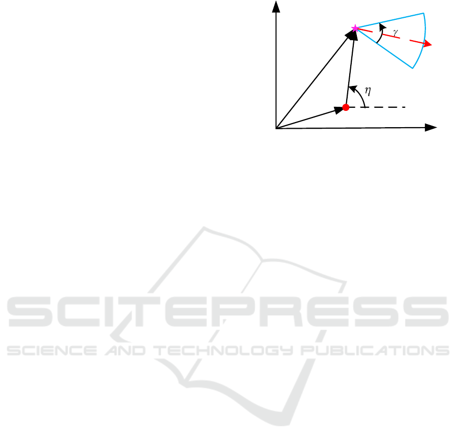
2.2 Measurement Model
Figure 1 shows the geometric relationship between
the observer and the target at time step k, where the
observer is represented by a magenta pentagram and
the red circle denotes the target. The red vector stands
for the observer heading direction at previous time
step. X −O −Y is the inertial coordinate. The no-
tations r
o,k
= [x
o,k
,y
o,k
]
T
and r
t,k
= [x
t,k
,y
t,k
]
T
repre-
sent the position vectors of the observer and the tar-
get at time step k, respectively. r
k
= r
o,k
−r
t,k
de-
notes the relative position vector between the observer
ICINCO 2019 - 16th International Conference on Informatics in Control, Automation and Robotics
92

and the target. η
k
denotes the bearing angle at cur-
rent time step, which represents the direction of the
relative position vector. With heading constraint (2),
the maximum region the observer can travel at current
time step is described by the blue sector with radius
V
o,max
T
s
and angle 2γ
max
, as shown in Fig. 1.
At time step k, the observer only has access to the
relative range provided by a range finder. Therefore,
the sensor measurement z
k
is given by
z
k
=
k
r
k
k
+ v
k
=
q
x
2
k
+ y
2
k
+ v
k
(3)
where v
k
denotes the sensor measurement noise,
which is assumed to be Gaussian white as v
k
∼
N

0,σ
2
r

with σ
r
being the standard deviation of the
measurement noise.
2.3 Problem Formulation
The objective of this paper is to analytically find an
one-step ahead optimal sensing strategy that min-
imises non-manoeuvring target localisation errors
with range-only measurements. For this optimisation
problem, we utilise the well-known FIM to formulate
the cost function since the inverse of FIM prescribes a
lower bound of the estimation error covariance of any
efficient estimator. Assume that the relative position
vector r
k
is known for finding the optimal observer
manoeuvre vector at time instant k. Then, the one-
step ahead position-related FIM for range-only local-
isation is given by
FIM =
1
σ
2
r
k+1
∑
i=k




∂
k
r
i
k
∂x
t,i

2
∂
k
r
i
k
∂x
t,i
∂
k
r
i
k
∂y
t,i
∂
k
r
i
k
∂x
t,i
∂
k
r
i
k
∂y
t,i

∂
k
r
i
k
∂y
t,i

2



=
1
σ
2
r
k+1
∑
i=k
"
cos
2
η
i
sin(2η
i
)
2
sin(2η
i
)
2
sin
2
η
i
#
(4)
For computational simplicity, we consider the deter-
minant of FIM, also known as D-optimality criterion,
as the cost function in our problem. The determinant
of FIM quantifies the volume of the estimation error
uncertainty ellipsoid and can be readily obtained from
Eq. (4) as
det(FIM) =
1
σ
4
r
sin
2
(η
k+1
−η
k
) (5)
Denote v
o,k
= [V
o,k
T
s
cosγ
o,k
.,V
o,k
T
s
sinγ
o,k
]
T
as the
observer manoeuvre vector at time step k and σ =
η
k+1
−η
k
. This paper formulates the following con-
strained discrete-time optimisation problem, denoted
as CDO
1
: find the observer manoeuvre vector at time
step k, v
o,k
, which maximises the following objective
function J
J = sin
2
σ (6)
subject to


γ
o,k
−γ
o,k−1


≤ ω
max
T
s
0 < V
o,k
≤V
o,max
(7)
The aim of this paper is to derive the closed-form
solution of CDO
1
.
3 DERIVATION OF OPTIMAL
SENSING STRATEGY FOR
ACTIVE TARGET
LOCALISATION
This section will propose an analytical optimal ma-
noeuvre that maximises the cost function J for target
localisation with range-only measurement. We first
derive the optimal solution without heading constraint
and then extend to the case that the robot has limited
turning rate to change its heading angle.
3.1 Optimal Solution without Heading
Constraints
Excluding the heading constraint, CDO
1
reduces to
CDO
2
: find the observer manoeuvre vector at time
step k, v
o,k
, which maximises the following objective
function J
J = sin
2
σ (8)
subject to
0 < V
o,k
≤V
o,max
(9)
Change in the vehicle’s velocity over a short interval,
like over T
s
, is usually negligible. Hence, for sim-
plicity, it is assumed that the observer moves with
constant speed and constant direction between two
consecutive time steps. Let v
t,k
=

v
tx,k
,v
ty,k

T
∆
=
[V
t,k
T
s
cosγ
t,k
,V
t,k
T
s
sinγ
t,k
]
T
be the target manoeuvre
vector at time step k. Assume that the target position
and velocity vector at current time step can be ob-
tained from Kalman filter, v
t,k
is known in trajectory
optimisation. Note that this assumption will be vali-
dated by a detailed observability analysis provided in
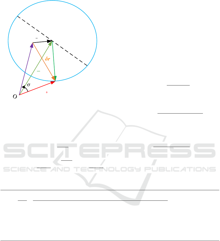
the next section. Figure 2 shows the geometric rela-
tionship between the observer and the target within
two consecutive time steps, where δr
k
represents the
relative manoeuvre at time step k and
¯
r
k
= r
k
−v
t,k
is an auxiliary vector utilised in the analysis. Since
v
t,k
is fixed,
¯
r
k
is known in trajectory optimisation.
The analytical solution of CDO
2
can be obtained us-
ing Lemmas 1 through 2.
Optimal Active Target Localisation Strategy with Range-only Measurements
93

r
k
k
1
r
k
,
v
o k
r
k
,
v
t k
Figure 2: Geometric illustration for moving target locali-
sation without turning rate limit in the relative frame. The
blue circle determines the maximum permissible region that
the observer can travel at current time step.
Lemma 1. Given the observer velocity V
o,k
, the can-
didate optimal heading angle at time step k without
any constraint is given by
γ
∗,1
o,k
= arcsin

−
V
o,k
T
s
k
¯
r
k
k

−ϑ (10)
γ
∗,2
o,k
= π −arcsin

−
V
o,k
T
s
k
¯
r
k
k

−ϑ (11)
with sin ϑ = b/
√
a
2
+ b
2
and cos ϑ = a/
√
a
2
+ b
2
,
where a = y
k
−v
ty,k
, b = x
k
−v
tx,k
.
Proof. For moving target, the relative manoeuvre
vector at time step k can be obtained as
δr
k
= v
o,k
−v
t,k
=

V
o,k
T
s
cosγ
o,k
−v
tx,k
,V
o,k
T
s
sinγ
o,k
−v
ty,k

T
(12)
Then, the relative position vector at time step k + 1 is
given by
r
k+1
= r
k
+ δr
k
= [x
k
+V
o,k
T
s
cosγ
o,k
−v
tx,k
,y
k
+V
o,k
T
s
sinγ
o,k
−v
ty,k
]
T
(13)
From Fig. 2, the separation angle σ between two
consecutive relative position vectors can be obtained
as
σ = arccos

r
T
k
·r
k+1
k
r
k
kk
r
k+1
k

(14)
Substituting Eq. (14) into Eq. (6) gives
J = 1 −cos
2
σ =
(x
k
y
k+1
−x
k+1
y
k
)
2

x
2
k
+ y
2
k

x
2
k+1
+ y
2
k+1

(15)
Since x
k
and y
k
are assumed to be known, max-
imising J is equivalent to maximising
¯
J =
(x
k
y
k+1
−x
k+1
y
k
)
2

x
2
k+1
+ y
2
k+1

(16)
Taking the partial derivative of
¯
J with respect to γ
o,k
and substituting Eq. (13) into it yields
∂
¯
J
∂γ
o,k
=
2V
o,k
T
s

x
k

y
k
−v
ty,k
+V
o,k
T
s
sinγ
o,k

−y
k
(x
k
−v
tx,k
+V
o,k
T
s
cosγ
o,k
)

h
(x
k
−v
tx,k
+V
o,k
T
s
cosγ
o,k
)
2
+

y
k
−v
ty,k
+V
o,k
T
s
sinγ
o,k

2
i
2
×
n
(x
k
cosγ
o,k
+ y
k
sinγ
o,k
)
h
(x
k
−v
tx,k
+V
o,k
T
s
cosγ
o,k
)
2
+

y
k
−v
ty,k
+V
o,k
T
s
sinγ
o,k

2
i
+

x
k

y
k
−v
ty,k
+V
o,k
T
s
sinγ
o,k

−y
k
(x
k
−v
tx,k
+V
o,k
T
s
cosγ
o,k
)

×

sinγ
o,k
(x
k
−v
tx,k
) −cos γ
o,k

y
k
−v
ty,k

(17)
Solving ∂
¯
J/∂γ
o,k
= 0 gives
x
k

y
k
−v
ty,k
+V
o,k
T
s
sinγ
o,k

−y
k
(x
k
−v
tx,k
+V
o,k
T
s
cosγ
o,k
) = 0
(18)

(x
k
−v
tx,k
)cosγ
o,k
+

y
k
−v
ty,k

sinγ
o,k
+V
o,k
T
s

×

x
2
k
+ y
2
k
−x
k
v
tx,k
−y
k
v
ty,k
+ x
k
V
o,k
T
s
cosγ
o,k
+y
k
V
o,k
T
s
sinγ
o,k
) = 0
(19)
Note that, if condition (18) is satisfied, e.g., the
observer heading results in the fact that the relative
manoeuvre vector δr
k
has either the same or the oppo-
site direction with r
k
, we have r
k+1
= λr
k
, λ ∈R. This
will minimises the cost function
¯
J as
¯
J = 0. Therefore,
this should be excluded from the solution candidates.
Together with the fact that the cost function
¯
J is con-
tinuous, the candidate optimal heading solutions can
be obtained from condition (19). Further simplifying
(19) yields

r
T
k+1
·v
o,k

r
T
k
·r
k+1

= 0 (20)
ICINCO 2019 - 16th International Conference on Informatics in Control, Automation and Robotics
94

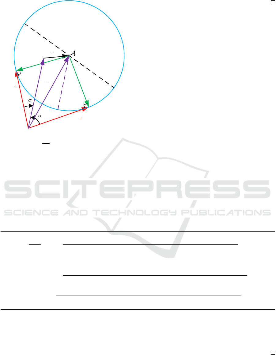
r
k
F
O
1
1
r
k
,
v
t k
*,1
,
v
o k
2
2
1
r
k
*,2
,
v
o k
1
r
k
Figure 3: Geometric illustration of the candidate optimal
heading solutions. AF is parallel to r
k
.
Since the optimal manoeuvre satisfies the condition
r
T
k
·r
k+1
6= 0, the final solution that locally maximises
¯
J is given by r
T
k+1
·v
o,k
= 0. This implies that the opti-
mal observer manoeuvre vector that maximises sin
2
σ
is perpendicular to next step relative position vector
r
k+1
. Using the definitions of r
k+1
and v
o,k
, we have
asinγ
o,k
+ bcosγ
o,k
= −V
o,k
T
s
(21)
Solving Eq. (21) for γ
o,k
gives Eqs. (10) and (11),
which completes the proof.
Remark 1. Given the robot velocity V
o,k
, Lemma 1
revels that there exist two locally optimal heading so-
lutions and these two solutions are symmetric with re-
spect to
¯
r
k
. The geometric illustration of the candidate
optimal solutions is presented in Fig. 3, where −v
t,k
is
assumed to be located on the right hand side of r
k
. It is
easy to verify that these two candidate heading direc-
tions provide the same level of optimality if
¯
r
k
= ρr
k
with ρ ∈ R, e.g., stationary target scenario or target
moves with either the same or the opposite direction
as r
k
. Except for these particular scenarios, there ex-
ists only one global optimal solution since σ
1
6= σ
2
.
Remark 2. Define γ
m
o,k
as the heading solution that
r
k+1
= λr
k
, λ ∈ R. Then, the proof of Lemma 1
indicates that, given the robot velocity V
o,k
, the cost
function monotonically increases when the heading
rotates from γ
m
o,k
to either γ
∗,1
o,k
or γ
∗,2
o,k
since there ex-
ists no solution of ∂
¯
J/∂γ
o,k
= 0 that locates between
γ
m
o,k
and γ
∗
o,k
. This property is useful in deriving the
optimal solution of the original optimisation problem.
The following lemma analyses the effect of ob-
server’s velocity on the cost function.
Lemma 2. If the heading angle satisfies condition
(10) or (11), the cost function J monotonically in-
creases with respect to the observer’s velocity V
o,k
.
Proof. Evaluate the partial derivative of
¯
J with re-
spect to V
o,k
and substitute r
T
k+1
·v
o,k
= 0 into it gives
∂
¯
J
∂V
o,k
= −2T
s

cosγ
o,k
(x
k
−v
tx,k
+V
o,k
T
s
cosγ
o,k
) + sin γ
o,k

y
k
−v
ty,k
+V
o,k
T
s
sinγ
o,k

(x
k
−v
tx,k
+V
o,k
T
s
cosγ
o,k
)
2
+

y
k
−v
ty,k
+V
o,k
T
s
sinγ
o,k

4
×

x
k
v
ty,k
−y
k
v
tx,k
+ T
s
V
o,k
y
k
cosγ
o,k
−T
s
V
o,k
x
k
sinγ
o,k

2
+ 2T
s
(y
k
cosγ
o,k
−x
k
sinγ
o,k
)

x
k
v
ty,k
−y
k
v
tx,k
+ T
s
V
o,k
y
k
cosγ
o,k
−T
s
V
o,k
x
k
sinγ
o,k

(x
k
−v
tx,k
+V
o,k
T
s
cosγ
o,k
)
2
+

y
k
−v
ty,k
+V
o,k
T
s
sinγ
o,k

2
=2T
s
(y
k
cosγ
o,k
−x
k
sinγ
o,k
)

x
k
v
ty,k
−y
k
v
tx,k
+ T
s
V
o,k
y
k
cosγ
o,k
−T
s
V
o,k
x
k
sinγ
o,k

(x
k
−v
tx,k
+V
o,k
T
s
cosγ
o,k
)
2
+

y
k
−v
ty,k
+V
o,k
T
s
sinγ
o,k

2
(22)
If v
∗
o,k
is located on the right hand side of r
k
(refer
to Fig. 3), we have
y
k
cosγ
o,k
−x
k
sinγ
o,k
> 0 (23)
and r
k+1
is located on the right hand side of r
k
, e.g.,
x
k

y
k
−v
ty,k
+V
o,k
T
s
sinγ
o,k

−y
k
(x
k
−v
tx,k
+V
o,k
T
s
cosγ
o,k
) < 0
(24)
Substituting Eqs. (23) and (24) into Eq. (22) yields
∂
¯
J/∂V
o,k
> 0. Similarly, one can easily verify that
∂
¯
J/∂V
o,k
> 0 when v
∗
o,k
is located on the left hand side
of r
k
. This implies that the cost function
¯
J monoton-
ically increases with the increase of observer’s veloc-
ity V
o,k
if the heading angle satisfies condition (10) or
(11), which completes the proof.
By using the results of Lemmas 1 and 2, the op-
timal observer manoeuvre, without any heading con-
straints, that maximises cost function J is obtained in
Optimal Active Target Localisation Strategy with Range-only Measurements
95

Theorem 1.
Theorem 1. The optimal solution of CDO
2
is given
by v
∗
o,k
=
h
V
o,max
T
s
cosγ
∗
o,k
,V
o,max
T
s
sinγ
∗
o,k
i
T
where
γ
∗
o,k
= max
γ
o,k
∈
n
γ
∗,1
o,k
,γ
∗,2
o,k
o
J (γ
o,k
) with
γ
∗,1
o,k
= arcsin

−
V
o,max
T
s
k
¯
r
k
k

−ϑ (25)
γ
∗,2
o,k
= π −arcsin

−
V
o,max
T
s
k
¯
r
k
k

−ϑ (26)
Proof. From Lemmas 1 and 2, the proof of Theorem
1 is straightforward.
Corollary 1. Under the proposed algorithm without
heading constraint, the relative range at next time
step is given by
k
r
k+1
k
=
q
k
¯
r
k
k
2
−(V
o,max
T
s
)
2
(27)
Proof. By definition of the relative range, we have
k
r
k+1
k
2
=

x
k
+V
o,max
T
s
cosγ
∗
o,k
−v
tx,k

2
+

y
k
+V
o,max
T
s
sinγ
∗
o,k
−v
ty,k

2
= (x
k
−v
tx,k
)
2
+

y
k
−v
ty,k

2
+ (V
o,max
T
s
)
2
+2V
o,max
T
s
h
(x
k
−v
tx,k
)cosγ
∗
o,k
+

y
k
−v
ty,k

sinγ
∗
o,k
i
(28)
Substituting Eq. (21) using V
o,max
into Eq. (28) leads
to the proof of Eq. (27).
Remark 3. From Corollary 1, one can note that the
relative range at next time step is influenced by the tar-
get moving speed and its direction. However, for lo-
calizing stationary target, the relative range is mono-
tonically decreasing. This is given by the following
corollary.
Corollary 2. Under the proposed algorithm without
heading constraint, the relative range monotonically
decreases with respect to time as
d
k
r
k
k
dt
= −
V
2
o,max
T
s
2
k
r
k
k
(29)
Proof. For stationary target, it is clear that
k
r
k
k
=
k
¯
r
k
k
. Then, Eq. (27) becomes
k
r
k+1
k
=
q
k
r
k
k
2
−(V
o,max
T
s
)
2
(30)
By definition, the rate of the relative range is deter-
mined by
d
k
r
k
k
dt
=
k
r
k+1
k
−
k
r
k
k
T
s
(31)
Substituting Eq. (31) into Eq. (30) and using V
o,max
yields
d
k
r
k
k
dt
=
q
k
r
k
k
2
−
(
V
o,max
T
s
)
2
−
k
r
k
k
T
s
=
k
r
k
k
s
1−
(
V
o,max
T
s
)
2
k
r
k
k
2
−
k
r
k
k
T
s
≈
k
r
k
k

1−
1
2
(
V
o,max
T
s
)
2
k
r
k
k
2

−
k
r
k
k
T
s
= −
V
2
o,max
T
s
2
k
r
k
k
(32)
3.2 Optimal Solution with Heading
Constraints
As discussed in Remark 1, if the target is stationary
or moves with either the same or the opposite di-
rection as r
k
, the candidate heading solutions, given
by Lemma 1, provide the same level of optimality.
This might generate multiple candidate trajectories
and zigzag heading change in practice. Therefore, it
is necessary to choose only one heading solution that
satisfies the practical heading change constraint when
implementing Theorem 1 in real applications. For this
reason, this subsection will propose the optimal solu-
tion of the constrained problem, e.g., CDO
1
.
Let γ
∗
o,k−1
be the optimal heading angle at
the previous time step. Without loss of gen-
erality, assume that γ
∗,1
o,k
is closer to γ
∗
o,k−1
than
γ
∗,2
o,k
, e.g.,



γ
∗,1
o,k
−γ
∗
o,k−1



≤



γ
∗,2
o,k
−γ
∗
o,k−1



. Denote
Ξ as the permissible heading angle set, e.g., Ξ
∆
=
n
γ
o,k



γ
∗
o,k−1
−γ
max
≤ γ
o,k
≤ γ
∗
o,k−1
+ γ
max
o
, then, the
solution of CDO
1
is determined as follows.
Condition 1: γ
∗,1
o,k
∈Ξ and γ
∗,2
o,k
∈Ξ. Under this con-
dition, the optimal heading angle is obviously given
by γ
∗
o,k
= max
γ
o,k
∈
n
γ
∗,1
o,k
,γ
∗,2
o,k
o
J (γ
o,k
). If these two candidate
heading solutions provide the same level of optimal-
ity, the heading direction, that is closer to previous
time step heading, is determined as the current head-
ing direction to generate a consistent and unique so-
lution, thus avoiding large heading change. With this
in mind, the optimal heading angle is given by
γ
∗
o,k
=





γ
∗,1
o,k
, if J

γ
∗,1
o,k

= J

γ
∗,2
o,k

max
γ
o,k
∈
n
γ
∗,1
o,k
,γ
∗,2
o,k
o
J (γ
o,k
), otherwise
(33)
Condition 2: γ
∗,1
o,k
∈ Ξ and γ
∗,2
o,k
/∈ Ξ. Since the
cost function monotonically increases when the head-
ing rotates from γ
m
o,k
to either γ
∗,1
o,k
or γ
∗,2
o,k
, the optimal
ICINCO 2019 - 16th International Conference on Informatics in Control, Automation and Robotics
96

heading solution is given by
γ
∗
o,k
= max
γ
o,k
∈
n
γ
∗,1
o,k
,
¯
γ
∗,1
o,k
,
¯
γ
∗,2
o,k
o
J (γ
o,k
) (34)
where
¯
γ
∗,1
o,k
= γ
∗
o,k−1
−γ
max
and
¯
γ
∗,2
o,k
= γ
∗
o,k−1
+ γ
max
.
Condition 3: γ
∗,1
o,k
/∈ Ξ and γ
∗,2
o,k
/∈ Ξ. Under this
condition, the optimal heading solution is obviously
located at the boundary of Ξ as
γ
∗
o,k
= max
γ
o,k
∈
n
¯
γ
∗,1
o,k
,
¯
γ
∗,2
o,k
o
J (γ
o,k
) (35)
Remark 4. Note that when γ
∗,2
o,k
is closer to γ
∗
o,k−1
than
γ
∗,1
o,k
, i.e.,



γ
∗,1
o,k
−γ
∗
o,k−1



>



γ
∗,2
o,k
−γ
∗
o,k−1



, similar re-
sults can also be obtained.
Remark 5. It is worthy pointing out that the ob-
server, under the proposed algorithm, will never col-
lide with the target since the minimum achievable rel-
ative range is limited by the turning rate constraint.
By summarizing the aforementioned three condi-
tions, the proposed active sensing strategy for target
localisation using range-only measurements is sum-
marized in Algorithm 1.
Algorithm 1 : Optimal Active Target localisation Strategy
with Range-Only Measurement.
Input: Estimated target position vector r
t,k
, estimated
target manoeuvre vector v
t,k
, previous observer ma-
noeuvre vector v
o,k−1
, maximum allowable heading
angle change γ
max
Output: Optimal observer heading angle γ
∗
o,k
1: Calculate the candidate optimal heading angles
γ
∗,1
o,k
and γ
∗,2
o,k
using Eqs. (25) and (26)
2: if



γ
∗,1
o,k
−γ
∗
o,k−1



≤



γ
∗,2
o,k
−γ
∗
o,k−1



then
3:
¯
γ
∗
o,k
= γ
∗,1
o,k
4: else
5:
¯
γ
∗
o,k
= γ
∗,2
o,k
6: end if
7: if



γ
∗,1
o,k
−γ
∗
o,k−1



≤ γ
max
and



γ
∗,2
o,k
−γ
∗
o,k−1



≤ γ
max
then
8: γ
∗
o,k
is given by Eq. (33)
9: else if



¯
γ
∗
o,k
−γ
∗
o,k−1



≤ γ
max
then
10: γ
∗
o,k
is given by Eq. (34)
11: else
12: γ
∗
o,k
is given by Eq. (35)
13: end if
4 OBSERVABILITY ANALYSIS
The baseline assumption that we utilised in deriving
the optimal heading solution is that current target po-
sition and velocity vector are available to the observer.
This information, however, is extracted from an esti-
mator in practical applications. For this reason, it is
necessary to analyse system observability since r
k
is
estimable only when target is observable. The results
are presented in the following proposition.
Proposition 1. Under the proposed algorithm, the
target is always observable.
Proof. The necessary and sufficient condition to
guarantee system observability for localising non-
manoeuvring target with range-only measurement is
given by (Song, 1999)
r(t) 6=

a
11
+ a
12
∆t
a
21
+ a
22
∆t

(36)
for some t ∈ (t
0
,t
f
] with t
0
being the initial time,
where ∆t = t −t
0
. The coefficients a
i j
in Eq. (36)
are arbitrary constants but not all zero.
If the target is unobservable, if follows from con-
dition (36) that there exists a line such that the relative
position always locates on the line with equal length
between two consecutive time steps, e.g., δr
i
= δr
j
,
∀i 6= j. This means that observer manoeuvre that
changes either the magnitude of the relative velocity
or the direction of the relative velocity is required for
range-only target localisation scenario. From previ-
ous analysis, we know that the proposed algorithm
leverages the maximum observer velocity and gen-
erates a unique solution that forces the relative po-
sition vector rotate either clockwise or anti-clockwise
around the target. Therefore, the direction of the rela-
tive velocity changes at every time instant, which im-
plies that there exists some t ∈ (t
k
,t
f
] such that con-
dition (36) is satisfied ∀t
k
. This means that target is
always observable under the proposed approach.
5 SIMULATION STUDIES
In this section, estimator-in-the-loop simulations are
performed to validate the proposed optimal sens-
ing strategy. The initial position of the robot is
(20m,50m) with initial heading 0
◦
. The maximum
permissible velocity of the robot is set as V
o,max
=
20m/s. The turning rate of the robot is constrained
by ω
max
= 1rad/s and the sampling time is set as
T
s
= 0.1s. The target initially locates at (0m, 0m) and
moves in a straight line with constant velocity V
t
=
5.83m/s as well as constant heading γ
t
= 0.54rad.
Optimal Active Target Localisation Strategy with Range-only Measurements
97

-50 0 50 100 150 200 250 300
X (m)
-50
0
50
100
150
200
Y (m)
Target
Numerical Optimization
Proposed Approach
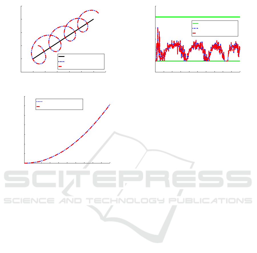
Figure 4: Moving trajectories.
0 5 10 15 20 25 30 35 40 45 50
Time (s)
0
2000
4000
6000
8000
10000
12000
14000
Determinant of FIM
Numerical Optimization
Proposed Approach
Figure 5: Determinant of FIM.
To implement the proposed algorithm, the required
information on target position and velocity are ex-
tracted from the well-known extended Kalman filter
in conjunction with a constant velocity model. For
validation, the numerical optimal solution of CDO
1
obtained from Particle Swarm optimisation algorithm
is also presented.
Figure 4 presents the moving trajectories of the
target and the observer. From this figure, one can
note that the proposed algorithm forces the relative
position vector rotate clockwise in the considered sce-
nario for target localisation. The determinant of FIM
is shown in Fig. 5, demonstrating that det(FIM) in-
creases monotonically with respect to time. Since
det(FIM) quantifies the volume of the estimation er-
ror uncertainty ellipsoid, target localisation perfor-
mance can be improved using the proposed active
sensing algorithm. Figure 6 provides the history of
observer’s heading rate, which reveals that the phys-
ical turning rate constraint is satisfied. Furthermore,
from the obtained results, we can clearly observe that
the proposed analytical solution coincides with the
numerical optimal solutions, demonstrating the effec-
tiveness of the proposed algorithm. Future work in-
cludes extending the proposed approach to heteroge-
neous sensors.
0 5 10 15 20 25 30 35 40 45 50
Time (s)
-1.5
-1
-0.5
0
0.5
1
1.5
Heading Rate (rad/s)
Turning Rate Limit
Numerical Optimization
Proposed Approach
Figure 6: Turning rate.
6 CONCLUSIONS
The problem of active target localisation using range-
only measurements is studied in this paper. By lever-
aging the determinant of one-step ahead FIM as the
cost function and heading angle command as the con-
trol input, the discrete-time optimal heading is de-
rived analytically to minimise target localisation error.
Both velocity and turning rate limits are considered in
the proposed optimisation approach. Numerical sim-
ulations are performed to validate the analytical finds.
REFERENCES
Atanasov, N., Le Ny, J., Daniilidis, K., and Pappas, G. J.
(2014). Information acquisition with sensing robots:
Algorithms and error bounds. In Robotics and Au-
tomation (ICRA), 2014 IEEE International Confer-
ence on, pages 6447–6454. IEEE.
Bajcsy, R., Aloimonos, Y., and Tsotsos, J. K. (2018).
Revisiting active perception. Autonomous Robots,
42(2):177–196.
Bishop, A. N., Fidan, B., Anderson, B. D., Do
˘
ganc¸ay,
K., and Pathirana, P. N. (2010). Optimality analysis
of sensor-target localization geometries. Automatica,
46(3):479–492.
Cao, Y. (2015). UAV circumnavigating an unknown tar-
get under a GPS-denied environment with range-only
measurements. Automatica, 55:150–158.
He, S., Shin, H.-S., and Tsourdos, A. (2019). Trajectory
optimisation for target localisation with bearing-only
measurement. IEEE Transactions on Robotics.
Logothetis, A., Isaksson, A., and Evans, R. J. (1997). An in-
formation theoretic approach to observer path design
for bearings-only tracking. In IEEE Conference on
Decision and Control, volume 4, pages 3132–3137.
IEEE.
Mart
´
ıNez, S. and Bullo, F. (2006). Optimal sensor place-
ment and motion coordination for target tracking. Au-
tomatica, 42(4):661–668.
ICINCO 2019 - 16th International Conference on Informatics in Control, Automation and Robotics
98

Matveev, A. S. and Semakova, A. A. (2017). Range-only
based 3d circumnavigation of multiple moving targets
by a non-holonomic mobile robot. IEEE Transactions
on Automatic Control.
Matveev, A. S., Semakova, A. A., and Savkin, A. V. (2016).
Range-only based circumnavigation of a group of
moving targets by a non-holonomic mobile robot. Au-
tomatica, 65:76–89.
Matveev, A. S., Teimoori, H., and Savkin, A. V. (2011).
Range-only measurements based target following for
wheeled mobile robots. Automatica, 47(1):177–184.
Salaris, P., Spica, R., Giordano, P. R., and Rives, P. (2017).
Online optimal active sensing control. In Robotics and
Automation (ICRA), 2017 IEEE International Confer-
ence on, pages 672–678. IEEE.
Song, T. L. (1999). Observability of target tracking with
range-only measurements. IEEE Journal of Oceanic
Engineering, 24(3):383–387.
Taylor, J. (1979). The cramer-rao estimation error lower
bound computation for deterministic nonlinear sys-
tems. IEEE Transactions on Automatic Control,
24(2):343–344.
Tokekar, P., Vander Hook, J., and Isler, V. (2011). Active
target localization for bearing based robotic teleme-
try. In Intelligent Robots and Systems (IROS), 2011
IEEE/RSJ International Conference on, pages 488–
493. IEEE.
Yang, Z., Shi, X., and Chen, J. (2014). Optimal coordina-
tion of mobile sensors for target tracking under addi-
tive and multiplicative noises. IEEE Transactions on
Industrial Electronics, 61(7):3459–3468.
Zhou, K., Roumeliotis, S. I., et al. (2011). Multirobot active
target tracking with combinations of relative observa-
tions. IEEE Transactions on Robotics, 27(4):678–695.
Optimal Active Target Localisation Strategy with Range-only Measurements
99