
Neural Networks Modelling of Aero-derivative Gas Turbine Engine:
A Comparison Study
Ibrahem M. A. Ibrahem
1
, Ouassima Akhrif
2
, Hany Moustapha
1
and Martin Staniszewski
3
1
Department of Mechanical Engineering, Ecole de Technologie Sup
´
erieure, 1100 Notre Dame St. W, Montreal, Canada
2
Department of Electrical Engineering, Ecole de Technologie Sup
´
erieure, 1100 Notre Dame St. W, Montreal, Canada
3
Digitalization Project Manager, Siemens Canada, 9545 Cote de Liesse Road, Montreal, Canada
martin.staniszewski@siemens.com
Keywords:
Neural Networks, NARX Model, Gas Turbine, Aero Derivative, Modelling, Simulation, Dynamic Neural
Networks.
Abstract:
In this paper, the modelling of aero derivative gas turbine engine with six inputs and five outputs using two
types of neural network is presented. Siemens three-spool dry low emission aero derivative gas turbine engine
used for power generation (SGT-A65) was used as a case study in this paper. Data sets for training and vali-
dation were collected from a high fidelity transient simulation program. These data sets represent the engines
operation above its idle status. Different neural network configurations were developed by using of a compre-
hensive computer code, which changes the neural networks parameters, namely, the number of neurons, the
activation function and the training algorithm. Next, a comparative study was done among different neural
models to find the most appropriate neural network structure in terms of computation time of neural network
training operation and accuracy. The results show that on one hand, the dynamic neural network has a higher
capability than the static neural network in representation of the engine dynamics. On the other hand however,
it requires a much longer training time.
1 INTRODUCTION
Aero-derivative gas turbine engines (ADGTE) are
widely used as a mechanical drive in oil and gas ap-
plication and power generation. These widespread
and increasing applications have sparked a great inter-
est among manufacturers to improve the performance
and increase the reliability of the engine, which in
turn requires an accurate and real time model to sim-
ulate the gas turbine engine dynamics. Siemens SGT-
A65 is a three spool ADGTE. The thermodynamic
physics based model for this engine configuration is
very complicated because of the high number of sub-
systems and the high number of non linear equations
that require to be solved iteratively at the expense of
computation time (Hanachi et al., 2015). This makes
it challenging if not impossible to use physics based
modelling approach in real time model based control
applications.
An alternative approach to physics based mod-
elling is data driven based modelling. Neural net-
works (NNs) is one of the data driven based (black
box) modelling approaches which can be used when
no or little information is available about the physics
of the system. It has the advantage of high computa-
tional speed allowing real time applications. The NN
model can be used in the development and operational
stages of an engine’s life to predict the engine’s per-
formance, test the performance of the engine control
systems and for engine health monitoring.
The main idea behind neural network modelling
is to create a simple model of human brain in order
to solve complex scientific and industrial problems in
many fields. Neural networks can be classified into
two main categories, static and dynamic neural net-
works. Static neural networks are the simplest neu-
ral networks, and are characterized by memoryless
non linear equations, which means that there are no
feedback elements and no delays in the network in-
put. Therefore, the output parameters from the static
NN depend only on the current values of the input pa-
rameters as shown in Fig. 1a. The multi layer feed
forward neural networks (MFFNN) are considered as
static neural networks because they have only feed
forward transformation of the information from the
input layer to the output layer.
738
Ibrahem, I., Akhrif, O., Moustapha, H. and Staniszewski, M.
Neural Networks Modelling of Aero-derivative Gas Turbine Engine: A Comparison Study.
DOI: 10.5220/0007928907380745
In Proceedings of the 16th International Conference on Informatics in Control, Automation and Robotics (ICINCO 2019), pages 738-745
ISBN: 978-989-758-380-3
Copyright
c
2019 by SCITEPRESS – Science and Technology Publications, Lda. All rights reserved

On the other hand, in the case of dynamic neu-
ral networks, output parameters from the network de-
pend not only on the current input parameters of the
network, but also on the previous input and output pa-
rameters of the network. Furthermore, dynamic neu-
ral networks can be divided into two categories: those
that have only feedforward connections (input/output
delays), and those that have feedback as shown in
Fig. 1b, or recurrent connections as shown in Fig. 1c.
(a) Static NN.
(b) Dynamic feed forward NN with input delay.
(c) Dynamic with feedback NN.
Figure 1: Neural network types(Beale et al., 2015).
There are many works in the literature regarding
the usage of static neural networks in modelling and
simulation of industrial gas turbine engines. (Laz-
zaretto and Toffolo, 2001), (Fast et al., 2009), (Asgari
et al., 2013) and (Rahmoune et al., 2015) are con-
sidered to be major research activities in this area.
These works are based on feed-forward NNs, with
a single hidden layer and different numbers of neu-
rons, trained by using a back propagation learning
algorithm. More recently, dynamic neural networks
have been employed for modelling gas turbine en-
gines. Non linear autoregressive network with exoge-
nous inputs (NARX) is a recurrent dynamic network,
with feedback connections enclosing several layers of
the network. (Salehi and Montazeri-Gh, 2018), (As-
gari et al., 2016) and (Bahlawan et al., 2017) used
NARX neural network to model ADGTE.
In this paper, a comparison study between MIMO
static feed forward neural network and MIMO NARX
dynamic neural networks was performed to model a
three spool ADGTE (SGT-A65) above its idle sta-
tus. A comprehensive computer program was used
for both types of NN to change the neural network
parameters, namely, the neuron number(from 1 to 20),
the activation function (tansig or logisg) as well as dif-
ferent training algorithms (trainlm, trainbr and train-
scg). After that, a comparative study was done among
different neural models to find the most appropriate
neural network structure in terms of training time and
accuracy by calculating the overall root mean square
error value.
2 AERO-DERIVATIVE GAS
TURBINE ENGINE
ADGTE are a popular choice for energy generation as
a result of their high reliability, efficiency and flexibil-
ity. ADGTE have also been widely used in pumping
applications for gas and oil transmission pipelines,
offshore platforms and naval propulsion. This kind
of gas turbines are derived from high bypass turbofan
engines. In this paper, a three spool dry low emis-
sion aero derivative gas turbine engine (SGT-A65)
was modelled as shown in Fig. 2. This engine con-
sists of two stages low axial low pressure compressor
(LPC), eight stages axial intermediate pressure com-
pressor (IPC), six stages axial high pressure compres-
sor (HPC), single stages high and intermediate tur-
bines and five stages low pressure turbine. The low
pressure shaft was connected with the power gener-
ator. Therefore, it should rotate at fixed revolution
(3600 rpm for electricity generation with 60 Hz).
The engine specifications are illustrated in Ta-
ble 1.
Figure 2: Siemens SGT-A65 aero derivative gas turbine en-
gine.
Table 1: Gas turbine technical data.
Parameter Value
Exhaust mass flow rate 171kg/s
Output power 65MW
Power turbine speed 3600rpm
Total compression ratio 38 : 1
Exhaust temperature 437
o
C
Neural Networks Modelling of Aero-derivative Gas Turbine Engine: A Comparison Study
739

3 NEURAL NETWORK
MODELLING METHOD
3.1 Available Field Data
In this paper, simulated data sets, which were used for
training and validation of the neural networks, were
provided to us by Siemens high fidelity transient sim-
ulation program for the SGT-A65 engine at ISO con-
ditions with a sampling rate of 0.1 sec. Note that,
the data was generated from a closed loop set-up with
Siemens own controller as the SGT-A65 engine can
not be run in open loop. Two sets of six inputs and
five outputs data were generated by changing the en-
gine load to cover the entire operating range of the
engine:
• Random load change (used for training) consist-
ing of 24170 samples;
• Square load change (used for validation) consist-
ing of 12890 samples;
As can be seen, a large number of training patterns
(samples) were used to train the NN. The number of
training patterns has an effect on the NN accuracy:
a low number of training patterns may increase the
NN error due to network over fitting. This means that
NN loses its ability to generalize. On the other hand,
this large number of training patterns may increase
the training computation time.
The SGT-A65 ADGTE input and output parame-
ters that are used, are illustrated in Table 2 and Table 3
respectively.
Table 2: The ADGTE input parameters.
Fuel flow G
f
LPC bleed off valve LPBOV
Variable inlet guide vans VIGV
IPC bleed off valve NBIP8
IPC variable stator vans IPVSV
HPC bleed off valve NBHP3
Table 3: The ADGTE output parameters.
Low-pressure shaft speed N
L
Intermediate shaft speed e N
I
High-pressure shaft speed N
H
Engine shaft power POWER
Intermediate turbine exit temperature TGT
Fig. 3 and Fig. 4 show the change of the normal-
ized input and output parameters for the SGT-A65
ADGTE used for training operation. Since the input
data to the NN represent the output from the engine
controller, the saturations in Fig. 3 are imposed by the
controller.
3.2 MIMO Static Neural Model
For this MIMO model, a feed forward multilayer
neural network was used to simulate the SGT-A65
ADGTE. This type of NN consists of an input layer
with a number of nodes equal to the number of in-
puts, one or more hidden layers with a certain num-
ber of neurons, and an output layer with a number of
neurons equal to the number of NN outputs. The first
parameter to be fixed is the number of hidden lay-
ers the static NN needs to have. Cybenco (Cybenko,
1989) proved that NN with one hidden layer of hyper-
bolic tangent or sigmoid activation function and one
output layer of linear activation function could simu-
late any non linear system. Therefore, in this study,
one hidden layer feed forward neural network was
used. To get an optimized neural network structure
which can represent the ADGTE dynamics, a com-
prehensive computer program was generated and run
in Matlab environment. This program generates dif-
ferent neural models by changing the following pa-
rameters:
• Change of the number of neurons from 1 to 20.
• Usage of two activation functions logsig and tan-
sig.
• Usage of three training algorithms: Levenberg-
Marquardt training algorithm (trainlm), Scaled
conjugate gradient training algorithm (trainscg)
and Bayesian regularization training algorithm
(trainbr).
At each computation cycle, training of the NN was
performed by using random load change data sets.
The stop network training parameters used are: (i)
the mean square error performance function which is
minimized until it reaches its minimum value (0.01),
(ii) the maximum number of training epochs (1000)
which represents the number of times that all the the
training patterns are presented to the NN and (iii) the
maximum number of validation increase (100) which
represents the number of successive epochs in which
the performance function fails to decrease. Training
operation was repeated three times for the same neu-
ral network with the same input data set to increase
the accuracy of the network. A preliminary analysis
which was carried out to evaluate the influence of
the number of training repetition showed that the
use of training repetition higher than three requires
a great computational effort, while it only allows a
small improvement of NN performance. Note that
the training operation was done in a computer with
ICINCO 2019 - 16th International Conference on Informatics in Control, Automation and Robotics
740

Figure 3: Normalized input parameters for model training.
Figure 4: Normalized output parameters for model training.
64 GB RAM and processor intel(R)Xeon(R) CPU
E3-1225 v6 @ 303GHz.
After that, validation of the trained network was
performed with another data set (Square load change
data set). The results of each computation cycle were
recorded in a matrix form which includes the network
structure, the root mean square error (RMSE) for
training process, RMSE for validation process and
training time. RMSE was used for the comparison of
the NNs. It was calculated for the whole set of data
of each output parameter from the NN, and defined
according to Eqn. (1),
RMSE =
s
1
n
n
∑
i=1
(
y
m
− y
y
m
)
2
(1)
where, n is the number of data samples, y
m
is the ac-
tual output and y is the predicted output. An over-
all RMSE of NN was also calculated as the sum of
RMSE of each output parameter.
To select the most appropriate static neural model
structure, the output data from the developed com-
puter program was divided into two groups as follows:
First Group. Static NNs with tansig activation func-
tion, different numbers of neurons and different train-
ing algorithms.
Neural Networks Modelling of Aero-derivative Gas Turbine Engine: A Comparison Study
741

Second Group. Static NNs with logsig activation
function, different numbers of neurons and different
training algorithms.
Next, the best NN from each group was selected
based on the minimum value of overall RMSE during
validation operation and minimum value of training
time. Fig. 5 shows the results analysis for first group
with respect to the overall value of the RMSE. Fig. 6
shows the results analysis for first group with respect
to the time consumed in the training phase.The results
of the second group are not shown for space reasons.
It can be noticed that the overall RMSE decreases
and the training time increases as number of neurons
in hidden layer increases. In particular, when NN
was trained by usage of trainlm or trainbr algorithms,
overall RMSE is smaller than overall RMSE of NN
trained by trainscg algorithm. On the other hand,
NNs trained by trainscg algorithm had the smallest
training time. However, the fast reduction in training
time by using (trainscg) was due to the fact that the
maximum number of validation increase was reached.
Table 4 summarizes the best result from each group.
As can be seen from Table 4 the best static MIMO
neural model configuration which can represent SGT-
A65 ADGTE should have eighteen neurons in the hid-
den layer, using tansig as activation function and us-
ing Levenberg-Marquardt (trainlm) as training algo-
rithm. In addition, the difference in the training time
between the best NN model in the first and second
group is small, which can be neglected in comparison
to network accuracy.
Figure 5: Influence of number of neurons with tansig acti-
vation function and different training algorithms.
Figure 6: Influence of number of neurons with tansig activa-
tion function and different training algorithms on the train-
ing time.
3.3 MIMO Dynamic Neural Model
There are many types of dynamic neural networks in
the literature (Norgaard et al., 2000). In this paper,
MIMO NARX recurrent dynamic neural network is
employed to simulate the SGT-A65 ADGTE, which
has feedback connections enclosing several layers of
the network. The following equation relates NARX
model output parameters to its input parameters,
y
i
(t) = f (y
i
(t − 1), y
i
(t − 2), · · · ,y
i
(t − n
y
)
,u
j
(t − 1), u
j
(t − 2), · · · ,u
j
(t − n
u
))
(2)
where, n
y
and n
u
are the number of regressed outputs
and regressed inputs respectively. These two param-
eters represent the most important parameters in the
NARX network configuration, and can be evaluated
by using system order estimation. In this study , we
used n
y
= 2 and n
u
= 2 based on the literature (Asgari
et al., 2016; Bahlawan et al., 2017).
Another important parameter in the NARX con-
figuration is the training architecture. The NARX net-
work training can be implemented via two architec-
tures:
Series-parallel Architecture (S&Pr) the network is
trained in open loop mode then transformed to
closed loop mode for validation operation.
Parallel Architecture (Pr) the network is trained
and validated in closed loop mode.
To get the optimal NARX model structure which
can represent the ADGTE dynamics, a comprehen-
sive computer program was generated and run in Mat-
lab environment. This program generates different
NARX models by changing the neural network pa-
rameters as shown in the static neural network for fair
comparison purposes. These parameters are as fol-
lows:
• Change of the number of neurons from 1 to 20.
• Usage of two activation functions logsig and tan-
sig.
• Usage of three training algorithms trainlm, train-
scg and trainbr.
• Train the network as series-parallel architecture
and parallel architecture.
The stop network training parameters are the same as
the ones for the MIMO static neural network, also the
training operation was performed on the same com-
puter as for MIMO static network. At each compu-
tation cycle, training of the NARX network was per-
formed by using random load change data set. After
that, validation for the trained network was performed
ICINCO 2019 - 16th International Conference on Informatics in Control, Automation and Robotics
742

Table 4: The best result from each group of MIMO static neural model.
No of neurons activation function training algorithm Testing RMSE training time
18 tansig trainlm 0.2388 25.404 sec
14 logsig trainlm 0.2475 17.844 sec
with another data set (Square load change data set).
The results of each computation cycle were recorded
in a matrix form which includes the network struc-
ture, RMSE for each output parameters in training
and validation phases, the overall root mean square
error RMSE for validation phase and training time.
The output data from the developed computer pro-
gram was divided into four groups as follows:
First Group: series-parallel NARX with tansig acti-
vation function, different numbers of neurons and dif-
ferent training algorithms [Fig. 7 and Fig. 8].
Second Group: series-parallel NARX with logsig ac-
tivation function, different numbers of neurons and
different training algorithms.
Third Group: parallel NARX with tansig activation
function, different numbers of neurons and different
training algorithms.
Fourth Group: parallel NARX with logsig activation
function, different numbers of neurons and different
training algorithms.
Figure 7: Influence of number of neurons with tansig acti-
vation function and different training algorithms.
Figure 8: Influence of number of neurons with tansig acti-
vation function and different training algorithms.
Note that, only figures from the first group will
be shown for space reasons. As can be seen, NARX
network with logsig activation function trained in par-
allel architecture with trainscg or trainbr algorithms
gave the best results with respect to the overall RMSE
values. However, this improvement in network accu-
racy came at the expense of increasing the training
time. On the other hand, the fast training time was
due to the stop of network training as the value of
maximum number of validation increase was reached.
Note also that the training time increases as the num-
ber of neurons in the hidden layer increases. More-
over, in a comparison of different structures of the
NARX NN, the results showed that the logsig acti-
vation function was superior to the tansig activation
function.
Table 5 summarizes the best result from each
group. As can be seen, the best MIMO NARX
model configuration which can represent SGT-A65
ADGTE should be a fourteen neurons in the hid-
den layer, using logsig as activation function and us-
ing Bayesian regularization (trainbr) as training algo-
rithm in the parallel architecture. This selected net-
work took much more time for training but made a
good prediction for all of the engine parameters, es-
pecially the low pressure spool speed (RMSE for low
pressure spool speed was 0.0009). On the other hand,
NARX network with eighteen neurons, tansig activa-
tion function, and trained in parallel architecture with
trainbr algorithm gave a lower training time than the
selected network. However, the RMSE for the low
pressure spool speed (0.0059) is higher than the one
in the selected network.
4 COMPARISON RESULTS
In this section, a comparison between the best MIMO
static neural model and the best MIMO NARX dy-
namic neural model was performed. Both MIMO
static neural model and MIMO NARX dynamic neu-
ral model were tested against the square data set. The
results are presented in Fig. 9 to Fig. 12 and summary
of these results was shown in Table 6. In a compari-
son of MIMO static NN with MIMO NARX dynamic
NN, the following results are obtained:
• The MIMO static NN and MIMO NARX dynamic
NN could represent the ADGTE with acceptable
accuracy.
• Eventhough the MIMO static NN has slightly
better performance (in term of overall RMSE)
than the MIMO NARX dynamic NN, the MIMO
NARX dynamic NN captures better the fast
Neural Networks Modelling of Aero-derivative Gas Turbine Engine: A Comparison Study
743

Table 5: The best result from each group of MIMO NARX model.
No of neurons activation function training algorithm S & PR / Pr Testing RMSE Training time
3 tansig trainscg S & PR 2.8760 1.7020 sec
18 logsig trainscg S & PR 1.1524 12.5930 sec
18 tansig trainbr Pr 0.3268 299.9670 sec
14 logsig trainbr Pr 0.3225 1333.9 sec
change in low pressure spool speed parameter,
high pressure spool speed, intermediate pressure
spool speed and intermediate turbine exit temper-
ature.
• The training time in the MIMO NARX dynamic
NN is higher than that in the MIMO static NN.
The increase in training time of the NARX net-
work may be due to the feedback connections and
the higher number of parameters which should be
evaluated during training phase.
• The generalization capability of the MIMO
NARX dynamic NN is higher than that in the
MIMO static NN.
• The MIMO static NN gave satisfactory results,
because a sufficient and adequate training data set
was used.
Figure 9: Variation of NH for the testing data.
Figure 10: Variation of NI for the testing data.
Dynamic networks are generally more powerful
than static networks. Therefore, the dynamic neural
networks can be used in multi step ahead prediction
applications. However, it takes much more training
time.
Figure 11: Variation of NL for the testing data.
Figure 12: Variation of TGT for the testing data.
Figure 13: Variation of power for the testing data.
5 CONCLUSIONS
In this paper, data driven modelling and identifica-
tion of Siemens SGT-A65 ADGTE is done using two
types of neural networks; static feed forward NN and
NARX dynamic NN. First, two sets of simulated data
from a high fidelity transient simulation program were
collected for training and validation process of the
networks. Second, selection of the best appropriate
neural model structure in both the static and dynamic
networks was performed by using a comprehensive
computer program, which changes the NN parameters
and performs training and validation of the produced
ICINCO 2019 - 16th International Conference on Informatics in Control, Automation and Robotics
744
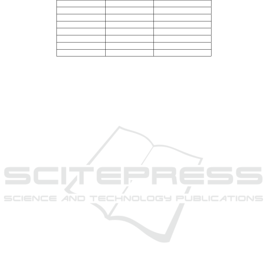
Table 6: Static and dynamic neural model comparison results.
Output parameter Static NN RMSE NARX model RMSE
N
L
0.01120 0.00098
N
I
0.00190 0.00039
N
H
0.00150 0.00047
POWER 0.21890 0.31890
TGT 0.00530 0.00170
Overall RMSE 0.23880 0.32250
Training time 25.404 sec 1333.9 sec
networks. The output data from this program were
recorded in a matrix form. After that, analysis of these
recorded data was performed by dividing the data into
different groups and selection of the best model struc-
ture from each group based on the minimum value
of RMSE. Finally, comparison results between static
NN and dynamic NN showed a good capability of the
dynamic neural networks over the static neural net-
works in representation of the dynamic response of
ADGTE. However, the training time of the dynamic
NN was higher than that in the static NN.
Since, there is no general methodology or rule to
define the neural network parameters, the way to se-
lect the best network configuration is traditionally ob-
tained by trial-and-error. This paper may work as
a guideline for researchers in selection of the best
feed forward and NARX neural network configura-
tion which can represent ADGTE during its full range
above its idle status.
In general, the developed NN models for the
ADGTE can be an effective tool for real time simu-
lation of gas turbines and model based control appli-
cations.
REFERENCES
Asgari, H., Chen, X., Menhaj, M. B., and Sainudiin, R.
(2013). Artificial neural network–based system identi-
fication for a single-shaft gas turbine. Journal of Engi-
neering for Gas Turbines and Power, 135(9):092601.
Asgari, H., Chen, X., Morini, M., Pinelli, M., Sainudiin,
R., Spina, P. R., and Venturini, M. (2016). Narx
models for simulation of the start-up operation of a
single-shaft gas turbine. Applied Thermal Engineer-
ing, 93:368–376.
Bahlawan, H., Morini, M., Pinelli, M., Spina, P. R., and
Venturini, M. (2017). Development of reliable narx
models of gas turbine cold, warm and hot start-up. In
ASME Turbo Expo 2017: Turbomachinery Technical
Conference and Exposition.
Beale, M. H., Hagan, M. T., and Demuth, H. B. (2015).
Neural network toolbox
TM
user’s guide. In R2015b,
The MathWorks, Inc., 3 Apple Hill Drive Natick, MA
01760-2098, , www.mathworks.com.
Cybenko, G. (1989). Approximation by superpositions of
a sigmoidal function. Mathematics of control, signals
and systems, 2(4):303–314.
Fast, M., Assadi, M., and De, S. (2009). Development and
multi-utility of an ann model for an industrial gas tur-
bine. Applied Energy, 86(1):9–17.
Hanachi, H., Liu, J., Banerjee, A., Chen, Y., and Koul, A.
(2015). A physics-based modeling approach for per-
formance monitoring in gas turbine engines. IEEE
Transactions on Reliability, 64(1):197–205.
Lazzaretto, A. and Toffolo, A. (2001). Analytical and neural
network models for gas turbine design and off-design
simulation. International Journal of Thermodynam-
ics, 4(4):173–182.
Norgaard, M., Ravn, O., Poulsen, N., and Hansen, L.
(2000). Neural networks for modelling and control
of dynamic systems: a practitioner’s handbook. Ad-
vanced textbooks in control and signal processing.
Springer, Berlin.
Rahmoune, M. B., Hafaifa, A., and Guemana, M. (2015).
Neural network monitoring system used for the fre-
quency vibration prediction in gas turbine. In Control,
Engineering & Information Technology (CEIT), 2015
3rd International Conference on, pages 1–5. IEEE.
Salehi, A. and Montazeri-Gh, M. (2018). Black box model-
ing of a turboshaft gas turbine engine fuel control unit
based on neural narx. Proceedings of the Institution of
Mechanical Engineers, Part M: Journal of Engineer-
ing for the Maritime Environment.
Neural Networks Modelling of Aero-derivative Gas Turbine Engine: A Comparison Study
745
