Using Network Traces to Generate Models for Automatic Network

Application Protocols Diagnostics

Martin Holkovi

, Ond

rej Ry

sav

and Libor Pol

CESNET a.l.e., Zikova 1903/4, 160 00 Prague, Czech Republic

Faculty of Information Technology, Brno University of Technology, Bozetechova 1/2, 612 66 Brno, Czech Republic

Keywords: Network Diagnostics, Automatic Diagnostics, Protocol Model from Traces.

Abstract:

Network diagnostics is a time-consuming activity that requires an administrator with good knowledge of net-

work principles and technologies. Even if some network errors have been resolved in the past, the administra-

tor must spend considerable time removing these errors when they reoccur. This article presents an automated

tool to learn the expected behavior of network protocols and possible variations. The created model can be

used to automate the diagnostic process. The model presents a ﬁnite automaton containing protocol behav-

ior for different situations. Diagnostics of unknown communication is performed by checking the created

model and searching for error states and their descriptions. We have also created a proof-of-concept tool that

demonstrates the practical potential of this approach.

1 INTRODUCTION

Computer networks consist of a large number of de-

vices and applications that communicate with each

other. Due to the complexity of the network, er-

rors occurred on a single device can negatively af-

fect the network services and thus the user experience.

There are various sources of error, such as miscon-

ﬁguration, poor connectivity, hardware error, or even

user misbehavior. End users are often unable to solve

these problems and seek help from a network admin-

istrator. The administrator must diagnose the current

situation, ﬁnd the cause of the problem, and correct it

to provide the service again.

The administrator diagnoses problems by check-

ing communication and ﬁnding possible causes

for these errors. Troubleshooting can be a rather

complex activity requiring good technical knowl-

edge of each network entity. Another complication

is that the administrator often has to check the number

of possible causes to ﬁnd the true source of the prob-

lem, which requires some time. Network problems

reappear even after the administrator detects and re-

solves these issues, such as repeating the same user

error or when the application update on the server

changes the expected behavior. All these problems

make the diagnostic process a time-consuming and

challenging activity that requires much administrator

attention.

(Zeng et al., 2012) provides a short survey that

shows that network diagnostics is time-consuming,

and administrators wish to have a more sophisticated

diagnostic tool available. Since each environment

is different, the use of universal tools is difﬁcult.

It would be useful to have a tool that adapts to be-

havior on a particular network. The tool should learn

the behavior of the network itself without the need

to program or specify rules on the behavior of indi-

vidual communicating applications and services.

Our goal is to develop a tool that automatically

creates a protocol behavior model. We are not aiming

at creating a general model for use in all networks, but

the model should describe diagnosed network only.

Instead of writing the model manually, the adminis-

trator provides examples (traces) of the protocol con-

versations in the form of PCAP ﬁles. The adminis-

trator provides two groups of ﬁles. The ﬁrst group

contains traces of normal behavior, while the second

group consists of known, previously identiﬁed error

traces. Based on these groups, the tool creates a proto-

col model. When the model is created, it can be used

for detection and diagnosis of issues in the observed

network communication. Once the model is created,

additional traces may be used to improve the model

gradually.

Our focus is on detecting application layer errors

in enterprise networks. Thus, in the presented work,

we do not consider errors occurred on other layers,

Holkovi

c, M., Ryšavý, O. and Pol

cák, L.

Using Network Traces to Generate Models for Automatic Network Application Protocols Diagnostics.

DOI: 10.5220/0007929900370047

In Proceedings of the 16th International Joint Conference on e-Business and Telecommunications (ICETE 2019), pages 37-47

ISBN: 978-989-758-378-0

e.g., wireless communication (Samhat et al., 2007),

routing errors (Dhamdhere et al., 2007), or perfor-

mance issue on the network layer (Ming Luo, 2011).

Because we are focusing on enterprise networks, we

make some assumption on the availability of required

source data. We expect that administrators using this

approach have access to network trafﬁc as the same

administrators operate the network infrastructure, and

it is possible to provide enough visibility to data

communication. Even the communication outside

the company’s network is encrypted, the trafﬁc be-

tween the company’s servers and inside the network is

many times unencrypted, or the data can be decrypted

by providing server’s private key or logging the sym-

metric session key

. Also, the source capture ﬁles

have no or minimal packet loss. An administrator can

recapture the trafﬁc if necessary.

When designing the system, we assumed some

practical considerations:

• no need to implement custom application protocol

dissectors;

• application error diagnostics cannot be affected

by lower protocols (e.g., version of IP protocol,

data tunneling protocol);

• easily readable protocol model - the created model

can be used for other activities too (e.g., security

analysis).

To demonstrate the potential of our approach,

we have created and evaluated a proof-of-concept im-

plementation available as a command line tool.

The main contribution of this paper is a new au-

tomatic diagnostic method for error detection in net-

work communication of commonly used application

protocols. The method creates a protocol behavior

model from packets traces that contain both correct

and error communication patterns. The administra-

tor can also use the created model for documentation

purposes and as part of a more detailed analysis,e.g.,

performance or security analysis.

This paper is organized as follows: Section 2 de-

scribes existing work comparable to the presented ap-

proach. Section 3 overviews the system architecture.

Section 4 provides details on the method, including

algorithms used to create and use a protocol model.

Section 5 presents the evaluation of the tool imple-

menting the proposed system. Finally, Section 6 sum-

marizes the paper and identiﬁes possible future work.

http://www.root9.net/2012/11/ssl-decryption-with-

wireshark-private.html

2 RELATED WORK

Recently published survey paper (Tong et al., 2018)

divides issues related to network systems as either

application-related or network-related problems. No-

table attention in troubleshooting of network appli-

cations was concentrated on networked multimedia

systems, e.g., (Leaden, 2007), (Shiva Shankar and

Malathi Latha, 2007), (Luo et al., 2007). Multimedia

systems require that certain quality of service (QoS)

is provided by the networking environment otherwise

various types of issues can occur. Network issues

comprise network reachability problems, congestion,

excessive packet loss, link failures, security policy vi-

olation, and router misconﬁguration.

Traditionally, network troubleshooting is a mostly

manual process that uses several tools to gather

and analyze relevant information. The ultimate tool

for manual network trafﬁc analysis and troubleshoot-

ing is Wireshark (Orzach, 2013). It is equipped with

a rich set of protocol dissectors that enables to view

details on the communication at different network

layers. An administrator has to manually analyze

the trafﬁc and decide which communication is abnor-

mal, possibly contributing to the observed problem.

Though Wireshark offers advanced ﬁltering mecha-

nism, it lacks any automation (El Sheikh, 2018).

Network troubleshooting employs active, passive,

or hybrid methods (Traverso et al., 2014). Ac-

tive methods rely on the tools that generate probing

packets to locate network issues (Anand and Akella,

2010). Specialized tools using generated diagnostic

communication were also developed for testing net-

work devices (Proch

azka et al., 2017). Contrary

to active methods, the passive approach relies only

on the observed information. Various data sources

can be mined to obtain enough evidence to identify

the problem. The collected information is then eval-

uated by the troubleshooting engine. The engine can

use different techniques of fault localization.

Rule-based systems describe normal and abnor-

mal states of the system. The set of rules is typic-

ally created by an expert and represents the domain

knowledge for the target environment. Rule-based

systems often do not directly learn from experience.

They are also unable to deal with new previously un-

seen situations, and it is hard to maintain the repre-

sented knowledge consistently (łgorzata Steinder and

Sethi, 2004).

Statistical and machine learning methods were

considered for troubleshooting misconﬁgurations

in home networks (Aggarwal et al., 2009) and diag-

nosis of failures in large Internet sites (Chen et al.,

2004). Tranalyzer (Burschka and Dupasquier, 2017)

DCNET 2019 - 10th International Conference on Data Communication Networking

Packets parser

Model training

Diagnostics

Data ﬁltering

Data pairing

Input data processing

Protocol model

PCAP ﬁle

Figure 1: After the system processes the input PCAP ﬁles (the ﬁrst yellow stage), it uses the data to create the protocol

behavior model (the second green stage) or to diagnose an unknown protocol communication using the created protocol

model (the-third purple stage).

is a ﬂow-based trafﬁc analyzer that performs trafﬁc

mining and statistical analysis enabling troubleshoot-

ing and anomaly detection for large-scale networks.

Big-DAMA (Casas et al., 2016) is another framework

for scalable online and ofﬂine data mining and ma-

chine learning supposed to monitor and characterize

extremely large network trafﬁc datasets.

Protocol analysis approach attempts to infer

a model of normal communication from data sam-

ples. Often, the model has the form of a ﬁnite automa-

ton representing the valid protocol communication.

An automatic protocol reverse engineering that stores

the communication patterns into regular expressions

was suggested in (Xiao et al., 2009). Tool ReverX

(Antunes et al., 2011) automatically infers a speciﬁ-

cation of a protocol from network traces and generates

corresponding automaton. Recently, reverse engi-

neering of protocol speciﬁcation only from recorded

network trafﬁc was proposed to infer protocol mes-

sage formats as well as certain ﬁeld semantics for bi-

nary protocols (Lodi et al., 2018).

3 SYSTEM ARCHITECTURE

This section describes the architecture of the proposed

system which learns from communication examples

and diagnoses unknown communications. The sys-

tem takes PCAP ﬁles as input data, where one PCAP

ﬁle contains only one complete protocol communi-

cation. An administrator marks PCAP ﬁles as cor-

rect or faulty communication examples before model

training. The administrator marks faulty PCAP ﬁles

with error description and a hint on how to ﬁx

the problem. The system output is a model describing

the protocol behavior and providing an interface for

using this model for the diagnostic process. The diag-

nostic process takes a PCAP ﬁle with unknown com-

munication and checks whether this communication

contains an error and if yes, returns a list of possible

errors and ﬁxes.

The architecture, shown in Figure 1, consists

of multiple components, each implementing a stage

in the processing pipeline. The processing is staged

as follows:

• Input Data Processing: Preprocessing is respon-

sible for converting PCAP ﬁles into a format suit-

able for the next stages. Within this stage, the in-

put packets are decoded using protocol parser.

Next, the ﬁlter is applied to select only relevant

packets. Finally, the packets are grouped to pair

request to their corresponding responses.

• Model Training: The training processes several

PCAP ﬁles and creates a model characterizing

the behavior of the analyzed protocol. The out-

put of this phase is a protocol model.

• Diagnostics: In the diagnostic component, an un-

known communication is analyzed and compared

to available protocol models. The result is a report

listing detected errors and possible hints on how

to correct them.

In the rest of the section, the individual compo-

nents are described in detail. Illustrative examples are

provided for the sake of better understanding.

3.1 Input Data Processing

This stage works directly with PCAP ﬁles provided

by the administrator. Each ﬁle is parsed by TShark

which exports decoded packets to JSON format.

The system further processes the JSON data by ﬁlter-

ing irrelevant records and pairs request packets with

their replies. The output of this stage is a list of tuples

representing atomic transactions.

3.1.1 Packets Parser

Instead of writing our packet decoders, we use

the existing implementation provided by TShark.

TShark is the console version of the well-known

Wireshark protocol analyzer which supports many

network protocols and can also analyze tunneled and

fragmented packets. In the case the Wireshark does

not support some protocol, e.g., proprietary, it is pos-

sible to use a tool which generates dissectors from

XML ﬁles (Golden and Coffey, 2015). The system

https://www.wireshark.org/docs/man-

pages/tshark.html

Using Network Traces to Generate Models for Automatic Network Application Protocols Diagnostics

...

"eth":{

"eth.dst":"f0:79:59:72:7c:30",

"eth.type":"0x00000800",

...

...

"dns":{

"dns.id":"0x00007956",

"dns.flags.response":"0",

"dns.flags.opcode":"0",

"dns.qry.name":"mail.patriots.in",

...

},

...

Figure 2: Excerpt from the TShark output into JSON for-

mat. The JSON represents POP3 packet values from all

network protocols in a key-value data format.

converts each input PCAP ﬁle into the JSON for-

mat (TShark supports multiple formats). The JSON

format represents data as a key-value structure (see

Figure 2), where the key is the name of the proto-

col ﬁeld according to Wireshark deﬁnition

, e.g.,

pop.request.command.

3.1.2 Data Filtering

The JSON format from the TShark output is still pro-

tocol dependent because the ﬁeld names are protocol-

dependent, and we have to know which key names

each protocol uses. The system converts the data

into a more generic format to make the next pro-

cessing protocol independent. We have found out,

that most of the application protocols use a request-

reply communication pattern. The system ﬁlters re-

quests and replies from each protocol and removes

the rest of the data. Even though the protocols use

the same communication pattern, they use a differ-

ent naming convention to mark the reply and response

values (see Table 1).

The problem is how to ﬁnd the requests and

replies in the JSON data. In our solution, we have

created a database of protocols and their processed

ﬁeld names. In the case the protocol is not yet in

the database, we require the administrator to add these

two ﬁeld names to the database. The administrator

can get the ﬁeld names from the Wireshark tool easily

by clicking on the appropriate protocol ﬁeld.

Messages can also contain additional informa-

tion and parameters, e.g., server welcome message.

The system also removes this additional information

to allow generalization of otherwise different mes-

sages during the protocol model creation. For exam-

https://www.wireshark.org/docs/dfref/

Table 1: Several application protocols with their request and

reply ﬁeld names with example values. The system takes

only data from these ﬁelds and drops the rest.

Name

Type Field name E.g.

SMTP

Request smtp.req.command MAIL

Reply smtp.response.code 354

FTP

Request ftp.request.command RETR

Reply ftp.response.code 150

POP

Request pop.request.command STAT

Reply pop.response.indicator +OK

DNS

Request dns.ﬂags.opcode 0

Reply dns.ﬂags.rcode 0

ple, the welcome server message often contains

the current date and time, which is always different,

and these different messages would create a lot of un-

repeatable protocol states. The Figure 3 shows the re-

sulting format from the Data ﬁltering step.

Unfortunately, TShark marks some unpredictable

data (e.g., authentication data) in some protocols as

regular requests and does not clearly distinguish it.

These values are a problem in later processing be-

cause these unpredictable values create ungeneraliz-

able states during the protocol model learning phase.

In our tests, we have observed that regular requests

have a maximal length of 6 characters, and unpre-

dictable requests have a much longer length. Based

on our ﬁnding, the system drops all requests that are

longer than six characters, and if necessary, the net-

work administrator can change this value. Distin-

guishing of these unpredictable requests also for other

protocols should be more focused in future research.

3.1.3 Data Pairing

To avoid pairing requests and replies during the pro-

tocol model learning process, the system pairs each

reply to its request in the data processing stage. After

this pairing process, the system represents each pro-

tocol with a list of pairs, each pair containing one

request and one reply. This pairing also simpli-

ﬁes the model learning process because some proto-

cols use the same reply value for multiple commands

(e.g., POP3 reply ”+OK” for all correct replies)

and the model could improperly merge several inde-

pendent reply values into one state (e.g., all POP3 suc-

cess replies jumps into one state).

The pairing algorithm iteratively takes requests

one by one and chooses the ﬁrst reply it ﬁnds.

If no reply follows, the system pairs the request with

a ”NONE” reply. In some protocols, the server sends

a reply to the client immediately after they connect

to the server. E.g., the POP server informs the clients

if it can process their requests or not. We have solved

this problem by pairing these replies with the empty

DCNET 2019 - 10th International Conference on Data Communication Networking

request ”NONE”. The result of the pairing process

is a sequence of pairs, where each pair consists of one

request and one reply. The Figure 3 shows an example

of this pairing process.

Data ﬁltering output Data pairing output

Reply: "220"

Request: "EHLO"

Reply: "250"

Request: "AUTH"

Reply: "334"

Reply: "235"

Request: "MAIL"

Reply: "250"

Request: "QUIT"

(None, "220")

("EHLO", "250")

("AUTH", "334")

("AUTH", "235")

("MAIL", "250")

("QUIT", None)

Figure 3: Example of an SMTP communication in which

the client authenticates, sends an email and quits the com-

munication. The left part of the example shows output from

the Data ﬁltering stage containing a list of requests and

replies in the protocol-independent format. The right part

shows a sequence of paired queries with replies, which are

the output of the Data pairing stage. The system pairs one

request and one reply with the special None value.

3.2 Model Training

After the Input Data Processing stage transformed in-

put PCAP ﬁles into a list of request-response pairs,

the Model Training phase creates a model of the pro-

tocol. The model has the form of a ﬁnite state

machine describing the behavior of the protocol.

The system creates the model from provided com-

munication traces. For example, for POP3 protocol,

we can consider regular communication traces that

represent typical operations, e.g., the client is check-

ing a mail-box on the server, downloading a message

from the server or deleting a message on the server.

The model is ﬁrst created for regular communication

and later extended with error behavior.

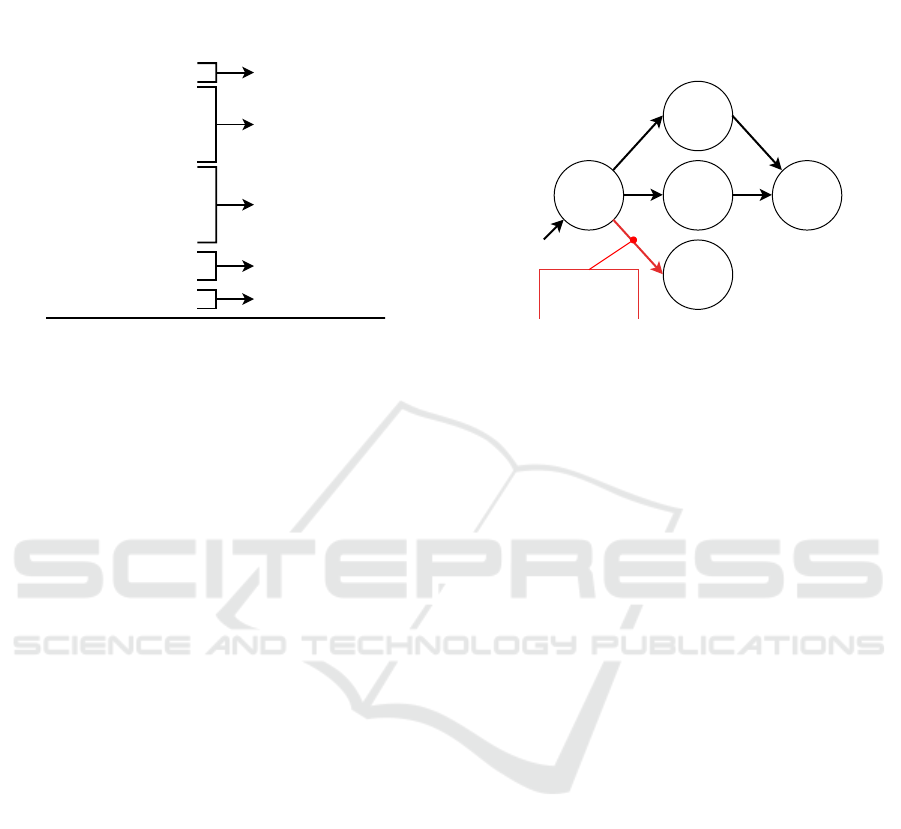
Learning from Traces with Expected Behavior.

The model creation process begins by learning

the protocol behavior from input data representing

regular communication. The result of this training

phase is a description of the protocol that represents

a subset of correct behavior. The model is created

from a collection of individual communication traces.

When a new trace is to be added, the tool identi-

ﬁes the longest preﬁx of the trace that is accepted

by the current model. The remaining of the trace

is then used to enrich the model. The Figure 4 shows

a simple example of creating a model from two cor-

rect communication traces (drawn in black ink).

1) CAPA, OK → STAT, OK → QUIT, OK

2) CAPA, OK → LIST, OK → QUIT, OK

3) CAPA, OK → STAT, ERR → QUIT, OK

error

description

CAPA,

+OK

QUIT,

+OK

STAT,

+OK

LIST,

+OK

STAT, -

ERR

CAPA,

+OK

QUIT,

+OK

QUIT,

+OK

LIST,

+OK

STAT,

-ERR

STAT,

+OK

Figure 4: An example of communication traces and the cor-

responding protocol model. The ﬁrst two sequences rep-

resent correct communication, while the third sequence

is communication with an error.

Learning the Errors.

After the system learns the protocol from regular

communication, the model can be extended with

error traces. In Figure 4, red arrow stands for a sin-

gle error transition in the model that corresponds

to the added error trace. The system expects that

the administrator prepares that error trace as the re-

sult of previous (manual) troubleshooting activities.

The administrator should also provide error descrip-

tion and information about how to ﬁx the error.

When extending the model with error traces,

the procedure is similar to when processing correct

traces. Automaton attempts to consume as long preﬁx

of input trace as possible ending in state s. The fol-

lowing cases are possible:

• Remaining input trace is not empty: The system

creates a new state s

and links it with from state

s. It marks the new state as an “error” state and

labels it with a provided error description.

• Remaining input trace is empty:

– State s is error state: The system adds the new

error description to existing labeling of an exis-

ting state s.

– State s is correct state: The system marks

the state as possible error and adds the error

description.

When extending the automaton with error traces,

it is possible that previously correct state is changed

to a possible error state. For consistent application

protocols, this ambiguity is usually caused by the ab-

Using Network Traces to Generate Models for Automatic Network Application Protocols Diagnostics

straction made when describing application protocol

behavior.

3.3 Diagnostics

After the system creates a behavioral model that is ex-

tended by error states, it is possible to use the model

to diagnose unknown communication tracks. The sys-

tem runs diagnostics by processing a PCAP ﬁle

in the same way as in the learning process and checks

the request/response sequence against the automaton.

Diagnostics distinguishes between these classes:

• Normal: the automaton accepts the entire input

trace and ends in the correct state.

• Error: the automaton accepts the entire input

trace and ends in the error state.

• Possible Error: the automaton accepts the en-

tire input trace and ends in the possible error

state. In this case, the system cannot distinguish

if the communication is correct or not. There-

fore, the system reports an error description from

the state and leaves the ﬁnal decision on the user.

• Unknown: the automaton does not accept en-

tire the input trace, which may indicate that

the trace represents a behavior not fully recog-

nized by the underlying automaton.

If the diagnostic process detects an unknown error

or result is not expected, the administrator must man-

ually analyze the PCAP ﬁle. After the administra-

tor decides whether the ﬁle contains an error or not,

the administrator should assign a ﬁle to a par-

ticular group of ﬁles (correct or error) and repeat

the learning process. This re-learning process in-

creases the model’s ability, and next time the sys-

tem sees the same situation, it reports the correct re-

sult. By gradually expanding, the model covers most

of the possible options.

4 ALGORITHMS

This section provides algorithms for (i) creating

a model from normal traces, (ii) updating the model

from error traces and (iii) evaluating a trace if it con-

tains an error. All three presented algorithms work

with a model that uses a deterministic ﬁnite automa-

ton (DFA) as its underlying representation.

The protocol behavior is an automaton

(Q,Σ,δ,q

,F). The set of states Q is represented

by all query/response pairs identiﬁed for the modeled

application protocol. As Q ⊆ Σ, the transition

relation δ : Q × Σ → Q is restricted as follows:

δ ⊆ {((q

),(q

))|(q

),(q

) ∈ Q}

Each state can be a ﬁnite state because the input

of the respective input is an indication of the state

reached and a list of error descriptions obtained when

processing the input data.

4.1 Adding Correct Traces

Algorithm 1 takes the current model (input variable

DFA) and adds missing transitions and states based

on the input sequence (input variable P). The al-

gorithm starts with the init state and saves it into

the previous state variable. The previous state vari-

able is used to create a transition from one state

to the next. In each loop of the while loop

section, the algorithm assigns the next pair into

the current state variable until there is no next

pair in the input. From the previous state and

the current state, the transition variable is created,

and the system checks if the DFA contains this tran-

sition. If the DFA does not contain the transition,

the transition is added to the DFA. Before continuing

with the next loop, the current state variable is as-

signed to the previous state variable. The updated

model will be used as the input for the next unpro-

cessed input sequence. After processing all the input

sequences, which represent normal behavior, the re-

sulting automaton is a model of normal behavior.

Algorithm 1: Updating model from the correct traces.

Inputs: P = sequence of query-reply pairs

DFA = set of the transitions

Output: DFA = set of the transitions

Previous state = init state

while not at end of input P do

Current state = get next pair from P

Transition = Previous state → Current state

if DFA does not contain Transition then

add Transition to DFA

Previous state = Current state

end

return DFA

4.2 Adding Error Traces

The Algorithm 2 has one more input (Error), which

is a text string describing a user-deﬁned error.

The start of the algorithm is the same as in the previ-

ous case. The difference is in testing whether the au-

tomaton contains the transition speciﬁed in the input

sequence. If so, the system checks to see if the saved

transition also contains errors. In this case, the al-

gorithm updates the error list by adding a new error.

Otherwise, the algorithm continues to process the in-

put string to ﬁnd a suitable place to indicate the error.

If the transition does not exist, i is created and marked

with the speciﬁed error.

DCNET 2019 - 10th International Conference on Data Communication Networking

Algorithm 2: Extending the model with error traces.

Inputs: P = sequence of query-reply pairs

DFA = set of transitions

Error = description of the error

Output: DFA = set of transitions

Previous state = init state

while not at end of input P do

Current state = get next pair from P

Transition = Previous state → Current state

if DFA contains Transition then

if Transition contains error then

append Error to Transition in DFA

return DFA

else

Previous state = Current state

else

add transition Transition to DFA

mark Transition in DFA with Error

return DFA

end

return DFA

4.3 Testing Unknown Trace

The Algorithm 3 uses previously created automa-

ton (DFA variable) to check the input sequence P.

According to the input sequence, the algorithm tra-

verses the automaton and collects the errors listed

in the transitions taken. If the required transition was

not found, the algorithm returns an error. In this case,

it is up to the user to analyze the situation and possibly

extend the automaton for this input.

5 EVALUATION

We have implemented a proof-of-concept tool which

implements the Algorithm 1, 2, and 3 speciﬁed

in the previous section. In this section, we pro-

vide the evaluation of our proof-of-concept tool

to demonstrate that the proposed solution is suit-

able for diagnosing application protocols. Another

goal of the evaluation is to show how the created

model changes by adding new input data to the model.

We have chosen four application protocols with dif-

ferent behavioral patterns for evaluation.

5.1 Reference Set Preparation

Our algorithms create the automata states and transi-

tions based on the sequence of pairs. The implica-

tion is that repeating the same input sequence does

not modify the learned behavior model. Therefore,

it is not important to provide a huge amount of in

put ﬁles (traces) but to provide unique traces (se-

quences of query-reply pairs). We created our refer-

ence datasets by capturing data from the network,

Algorithm 3: Checking an unknown trace.

Inputs: P = sequence of query-reply pairs

DFA = set of transitions

Output: Errors = one or more error descriptions

Previous state = init state

while not at end of input P do

Current state = get next pair from P

Transition = Previous state → Current state

if DFA contains Transition then

if Transition contains error then

return Errors from Transition

else

Previous state = Current state

else

return ”unknown error”

end

return ”no error detected”

removing unrelated communications, and calculating

the hash value for each trace to avoid duplicate pat-

terns. Instead of a correlation between the amount

of protocols in the network and the amount of saved

traces, the amount of ﬁles correlates with the com-

plexity of the analyzed protocol. For example,

hundreds of DNS query-reply traces captured from

the network can be represented by the same sequence

(dns query, dns reply).

After capturing the communication, all the traces

were manually checked and divided into two groups:

(i) traces representing normal behavior and (ii) traces

containing some error. In case the trace contains

an error, we also identiﬁed the error and added

the corresponding description to the trace. We split

both groups of traces (with and without error) into

the training set and the testing set.

It is also important to notice that the tool uses

these traces to create a model for one speciﬁc (or sev-

eral) network conﬁguration and not for all possible

conﬁgurations. Focus on a single conﬁguration re-

sults in a smaller set of unique traces and smaller cre-

ated models. This focus allows an administrator to

detect situations which may be correct for some net-

work, but it is not correct for a diagnosed network,

e.g., missing authentication.

5.2 Model Creation

We have chosen the following four request-reply ap-

plication protocols with different complexity for eval-

uation:

• DNS: Simple stateless protocol with simple com-

munication pattern - domain name query (type A,

AAAA, MX, ...) and reply (no error, no such

name, ...).

• SMTP: Simple state protocol in which the client

has to authenticate, specify email sender and re-

cipients, and transfer the email message. The pro-

Using Network Traces to Generate Models for Automatic Network Application Protocols Diagnostics

Table 2: For each protocol, the amount of total and training traces is shown. These traces are separated into successful

(without error) and failed (with error) groups. The training traces are used to create two models, the ﬁrst without errors and

the second with errors. The states and transitions columns indicate the complexity of the created models.

Protocol

Total traces Training traces

Model without

error states

Model with

error states

Successful Failed Successful Failed States Transitions States Transitions

DNS 16 8 10 6 18 28 21 34

SMTP 8 4 6 3 11 18 14 21

POP 24 9 18 7 16 44 19 49

FTP 106 20 88 14 33 126 39 137

tocol has a large predeﬁned set of reply codes re-

sulting in many possible states in DFA created

by Algorithm 1 and 2.

• POP: In comparison with SMTP, from one point

of view, the protocol is more complicated be-

cause it allows clients to do more actions with

email messages (e.g., download, delete). How-

ever, the POP protocol replies only with two pos-

sible replies (+OK, -ERR), which reduce the num-

ber of possible states.

• FTP: It is stateful protocol usually requires

authentication, then allows the client to do mul-

tiple actions with ﬁles and directories, and also

the protocol deﬁnes many reply codes.

The proof-of-concept tool took input data of se-

lected application protocols and created models

of the behavior without errors and a model with er-

rors. The Table 2 shows the distribution of the input

data into a group of correct training traces and a group

of traces with errors. Remaining traces will be later

used for testing the model. The right part of the ta-

ble shows the complexity of the generated models

in the format of states and transitions count.

Based on the statistics of models, we have made

the following conclusions:

• transitions count represents the complexity

of the model better than the state’s count;

• there is no direct correlation between the com-

plexity of the protocol and the complexity

of the learned model. As can be seen with pro-

tocols DNS and SMTP, even though the model

SMTP is more complicated than DNS protocol,

there were about 50% fewer unique traces result-

ing in a model with 21 transitions, while the DNS

model consists of 34 transitions. The reason

for this situation is that one DNS connection can

contain more than one query-reply and because

the protocol is stateless, any query-reply can fol-

low the previous query-reply value.

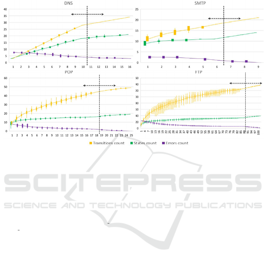
Figure 5 shows four charts of four protocols

that show the complexity of the models in terms

of the number of states, transitions, and testing traces

with error results. Each chart consists of two parts.

The ﬁrst part marked as training from correct traces

creates the model only from traces without errors.

To check the correctness of the model, we used testing

traces with and without errors. The second part learn-

ing the errors takes the model created from all the suc-

cessful traces and extends it with training traces with

known errors. To mark the testing trace without

error as a correct result, the model has to return that

the trace is without error. Testing traces with an error

are marked as correct when an error was detected, and

the model found the correct error description.

The charts in Figure 5 shows the progress

of changing the model size when new traces are added

to the model. We have created these values from

25 tests, and the charts show a range of the values

from these tests with their median. Each test be-

gan by randomizing the order of the trace ﬁles, re-

sulting in a different trace order in each test. Based

on the deviation of values from the median, we can

see that during the learning process, the model is de-

pendent on the order of the traces. However, after

we have added all the traces, the created model has

the same amount of states and transitions (zero de-

viation). The zero deviation can be seen at the end

of training from correct trace states and also at the end

of learning the error states. We have also used

a diff tool to compare the ﬁnal models between them-

selves to conﬁrm that all the models were the same,

and the ﬁnal model does not depend on the order

of the input traces.

Figure 5 shows that by adding new traces, the size

of the model is increasing. With the increasing

size of the model, the model is more accurate, and

the amount of diagnostic error results decreases.

However, after some amount of traces, the model ex-

pansion will slow down until it stops after the tool has

observed all valid traces. Stopping the expansion may

seem like the point when the model is fully trained,

however from our experience, it is not possible to de-

termine when the model is fully learned or at least

DCNET 2019 - 10th International Conference on Data Communication Networking

learning

the errors

training from correct traces

training from correct traces learning the errors

training from correct traces

learning the errors

training from correct traces

traces traces

traces

126

137

Figure 5: The ﬁgure shows the count of transitions, states, and errors in the four analyzed protocols. An error is an incorrect

diagnostic result. The values are extracted from 25 random tests, and the median of their values is represented by intercon-

nection lines. The learning process is split into two parts: i) training the model only from traces without any error and after

all correct traces have been learned, in section ii) model is extended with the knowledge of known errors.

learned from X%. Even if the model does not grow

for a long time, it can suddenly expand by processing

a new trace (new extensions, programs with speciﬁc

behavior, program updates).

Another way of specifying how much percent

the model is trained is by calculating all possi-

ble transitions. The calculation is (requests count ∗

replies count)

. Of course, many combinations

of requests and replies would not make any sense,

but the algorithm can never be sure which combina-

tions are valid and which are not. The problem with

counting all possible combinations is that without pre-

deﬁned knowledge of diagnosed protocol the tool can

never be sure if all possible requests and replies (no

matter the combinations) have already be seen or not.

5.3 Evaluation of Test Traces

Table 3 shows the amount of successful and failed

testing traces; the right part of Table 3 shows testing

results for these data. All tests check whether:

1. a successful trace is marked as correct (TN);

2. a failed trace is detected as an error trace with cor-

rect error description (TP);

3. a failed trace is marked as correct (FN);

4. a successful trace is detected as an error or failed

trace is detected as an error but with an incorrect

error description (FP);

5. true/false (T/F) ratios which are calculated

as (T N + T P)/(FN + FP). T/F ratios represents

how many traces the model diagnosed correctly.

As the columns T/F ratio in Table 3 shows, most

of the testing data was diagnosed correctly. We have

analyzed the incorrect results and made the following

conclusions:

• DNS: False positive - One application has made

a connection with the DNS server and keeps

the connection up for a long time. Over

time several queries were transferred. Even

though the model contains these queries, the or-

der in which they came is new to the model.

The model returned an error result even when

the communication ended correctly. An incom-

plete model causes this misbehavior. To correctly

diagnose all query combinations, the model has

to be created from more unique training traces.

• DNS: False positive - The model received a new

SOA update query. Even if the communication

did not contain the error by itself, it is an indica-

tion of a possible anomaly in the network. There-

fore, we consider this as the expected behavior.

• DNS: False negative - The situation was the same

as with the ﬁrst DNS False positive mistake -

Using Network Traces to Generate Models for Automatic Network Application Protocols Diagnostics

Table 3: The created models have been tested by using testing traces, which are split into successful (without error) and

failed (with error) groups. The correct results are shown in the true negative and true positive columns. The columns false

positive and false negative on the other side contain the number of wrong test results. The ratio of correct results is calculated

as a true/false ratio. This ratio represents how many testing traces were diagnosed correctly.

Protocol

Testing traces

Testing against model

without error states

Testing against model

with error states

Successful Failed TN TP FN FP T/F ratio TN TP FN FP T/F ratio

DNS 6 2 4 2 0 2 75 % 4 1 1 2 63 %

SMTP 2 1 2 1 0 0 100 % 2 1 0 0 100 %

POP 6 2 6 2 0 0 100 % 6 2 0 0 100 %

FTP 18 6 18 6 0 0 100 % 18 5 1 0 96 %

TN - true negative, TP - true positive, FN - false negative, FP - false positive, T/F ratio - true/false ratio

the order of packets was unexpected. Unex-

pected order resulted in an unknown error instead

of an already learned error.

• FTP: False negative - The client sent a PASS

command before the USER command. This

resulted in an unexpected order of commands,

and the model detected an unknown error. We are

not sure how this situation has happened, but be-

cause it is nonstandard behavior, we are inter-

preting this as an anomaly. Hence, the proof-of-

concept tool provided the expected outcome.

All the incorrect results are related to the incom-

plete model. In the real application, it is almost im-

possible to create a complete model even with many

input data. In the stateless protocols (like DNS),

it is necessary to capture traces with all combinations

of query-reply states. For example, if the protocol de-

ﬁnes 10 types of queries, 3 types of replies, the to-

tal amount of possible transitions is (10 ∗ 3)

= 900.

Another challenge is a protocol which deﬁnes many

error reply codes. To create a complete model, all

error codes in all possible states need to be learned

from the traces.

We have created the tested tool as a prototype

in Python language. We have not aimed at testing

the performance, but to get at least an idea of how us-

able our solution is, we gathered basic time statistics.

The processing time of converting one PCAP ﬁle (one

trace) into a sequence of query-replies and adding it

to the model took on average 0.4s. This time had only

small deviations because most of the time took ini-

tialization of the TShark. The total amount of time

required to learn a model depends on the amount

of PCAPs. The average time required to create

a model from 100 PCAPs was 30 seconds.

6 CONCLUSIONS

This paper suggested a method for automatic error

diagnostics in network application protocols by cre-

ating models for these applications. There are two

use-cases for when administrators should use this ap-

proach: (i) if an administrator is experienced, the ad-

ministrator can learn the model to speed-up the diag-

nostic process; (ii) if an administrator is inexperi-

enced, the administrator can use the model created by

an experienced administrator to diagnose the network.

The already existing diagnostic solutions do not

have any automation capabilities, require an adminis-

trator to create rules describing the normal and error

states or the automatically created protocol models

are not used for diagnostic purposes.

Our method uses network traces prepared by ad-

ministrators to create a model representing proto-

col behavior. The administrator has to separate the

correct from the error traces and annotate the error

ones. The model is created based on the query-

response sequences extracted from the analyzed pro-

tocol. For this reason, the model is applicable only

for a protocol with a query-reply pattern. The model

represents the correct and incorrect protocol behavior,

which is used for unknown network trace diagnostics.

The main beneﬁt of having an own trained model

is that the model will represent the protocol in a spe-

ciﬁc conﬁguration and will not accept situations

which may be valid only for other networks. The ad-

ministrator can use the model to speed up the work

by automating unknown communication diagnostics.

Our solution uses the well-known tool TShark, which

supports many network protocols and allows us to use

the Wireshark display language to mark the data.

We have implemented the proposed method

as a proof-of-concept tool

to demonstrate its capa-

bilities. The tool has been tested on four application

https://github.com/marhoSVK/semiauto-diagnostics

DCNET 2019 - 10th International Conference on Data Communication Networking

protocols that exhibit different behavior. Experiments

have shown that it is not easy to determine when

a model is sufﬁciently taught. Even knowing the pro-

tocol complexity is not a reliable indication. Because

even the simplest protocol we tested needed a larger

model than a more complex protocol. Although the

model seldom covers all possible situations, it is use-

ful for administrators to diagnose repetitive and typi-

cal protocol behavior and ﬁnd possible errors.

Future work will focus on: (i) ﬁnding other au-

tomation cases for the created protocol model ; (ii) de-

signing and implementing additional communication

modeling algorithms to support other useful commu-

nication features ; (iii) a study on possibility of com-

bining different models from multiple algorithms into

one complex model; (iv) integrating timing informa-

tion into DFA edges.

ACKNOWLEDGEMENTS

This work was supported by project ”Network Diag-

nostics from Intercepted Communication” (2017-

2019), no. TH02010186, funded by the Tech-

nological Agency of the Czech Republic and by BUT

project ”ICT Tools, Methods and Technologies for

Smart Cities” (2017-2019), no. FIT-S-17-3964.

REFERENCES

Aggarwal, B., Bhagwan, R., Das, T., Eswaran, S., Padman-

abhan, V. N., and Voelker, G. M. (2009). NetPrints:

Diagnosing home network misconﬁgurations using

shared knowledge. Proceedings of the 6th USENIX

symposium on Networked systems design and imple-

mentation, Di(July):349–364.

Anand, A. and Akella, A. (2010). {NetReplay}: a new

network primitive. ACM SIGMETRICS Performance

Evaluation Review.

Antunes, J., Neves, N., and Verissimo, P. (2011). Reverx:

Reverse engineering of protocols. Technical Report

2011-01, Department of Informatics, School of Sci-

ences, University of Lisbon.

Burschka, S. and Dupasquier, B. (2017). Tranalyzer: Ver-

satile high performance network trafﬁc analyser. In

2016 IEEE Symposium Series on Computational In-

telligence, SSCI 2016.

Casas, P., Zseby, T., and Mellia, M. (2016). Big-DAMA:

Big Data Analytics for Network Trafﬁc Monitoring

and Analysis. Proceedings of the 2016 Workshop on

Fostering Latin-American Research in Data Commu-

nication Networks (ACM LANCOMM’16).

Chen, M., Zheng, A., Lloyd, J., Jordan, M., and Brewer, E.

(2004). Failure diagnosis using decision trees. Inter-

national Conference on Autonomic Computing, 2004.

Proceedings., pages 36–43.

Dhamdhere, A., Teixeira, R., Dovrolis, C., and Diot, C.

(2007). NetDiagnoser: Troubleshooting network un-

reachabilities using end-to-end probes and routing

data. Proceedings of the 2007 ACM CoNEXT.

El Sheikh, A. Y. (2018). Evaluation of the capabilities of

wireshark as network intrusion system. Journal of

Global Research in Computer Science, 9(8):01–08.

Golden, E. and Coffey, J. W. (2015). A tool to automate

generation of wireshark dissectors for a proprietary

communication protocol. The 6th International Con-

ference on Complexity, Informatics and Cybernetics,

IMCIC 2015.

Leaden, S. (2007). The Art Of VOIP Troubleshooting. Busi-

ness Communications Review, 37(2):40–44.

łgorzata Steinder, M. and Sethi, A. S. (2004). A survey

of fault localization techniques in computer networks.

Science of computer programming, 53(2):165–194.

Lodi, G., Buttyon, L., and Holczer, T. (2018). Message

Format and Field Semantics Inference for Binary Pro-

tocols Using Recorded Network Trafﬁc. In 2018 26th

International Conference on Software, Telecommuni-

cations and Computer Networks, SoftCOM 2018.

Luo, C., Sun, J., and Xiong, H. (2007). Monitoring and

troubleshooting in operational IP-TV system. IEEE

Transactions on Broadcasting, 53(3):711–718.

Ming Luo, Danhong Zhang, G. P. L. C. (2011). An in-

teractive rule based event management system for

effective equipment troubleshooting. Proceedings

of the IEEE Conference on Decision and Control,

8(3):2329–2334.

Orzach, Y. (2013). Network Analysis Using Wireshark

Cookbook. Packt Publishing Ltd.

Proch

azka, M., Macko, D., and Jelemensk

a, K. (2017). IP

Networks Diagnostic Communication Generator. In

Emerging eLearning Technologies and Applications

(ICETA), pages 1–6.

Samhat, A., Skehill, R., and Altman, Z. (2007). Automated

troubleshooting in WLAN networks. In 2007 16th IST

Mobile and Wireless Communications Summit.

Shiva Shankar, J. and Malathi Latha, M. (2007). Trou-

bleshooting SIP environments. In 10th IFIP/IEEE In-

ternational Symposium on Integrated Network Man-

agement 2007, IM ’07.

Tong, V., Tran, H. A., Souihi, S., and Mellouk, A. (2018).

Network troubleshooting: Survey, Taxonomy and

Challenges. 2018 International Conference on Smart

Communications in Network Technologies, SaCoNeT

2018, pages 165–170.

Traverso, S., Tego, E., Kowallik, E., Raffaglio, S., Fregosi,

A., Mellia, M., and Matera, F. (2014). Exploiting hy-

brid measurements for network troubleshooting. In

2014 16th International Telecommunications Network

Strategy and Planning Symposium, Networks 2014.

Xiao, M. M., Yu, S. Z., and Wang, Y. (2009). Automatic

network protocol automaton extraction. In NSS 2009

- Network and System Security.

Zeng, H., Kazemian, P., Varghese, G., and McKeown, N.

(2012). A survey on network troubleshooting. Tech-

nical Report Stanford/TR12-HPNG-061012, Stanford

University, Tech. Rep.

Using Network Traces to Generate Models for Automatic Network Application Protocols Diagnostics