Computation of Trajectory Sensitivities with Respect to Control and

Implementation in PSAT

Ramij Raja Hossain

and Ratnesh Kumar

Department of Electrical and Computer Engineering, Iowa State University, Ames, Iowa 50011, U.S.A.

Keywords:

Power System, PSAT, Static VAR Compensator, Trajectory Sensitivity wrt Control, Under Load Tap Changer.

Abstract:

Trajectory sensitivity based analysis is widely regarded as an important tool for real time protection scheme

of power systems. Model Predictive Control (MPC) for voltage instability is one such protection scheme

which computes a sequence of control actions depending upon the trajectory behaviour of the dynamics of the

power systems. Thus, computation of trajectory sensitivities with respect to control input can be an integral

part for designing a real-time protection scheme. In this context, it is important to note that for the state-

of-the-art Power System Analysis Tool (PSAT)(Milano, 2005), (Milano et al., 2008), while it is relatively

easy to compute the trajectory sensitivities with respect to any system variables, the computation of trajectory

sensitivities with respect to control inputs is not explicitly supported. This paper presents a method to extend

the functionality of PSAT to also compute the trajectory sensitivities with respect to control inputs, which

ultimately forms the basis for real-time protection schemes such as MPC. The proposed method is validated

using direct time-domain simulation results.

1 INTRODUCTION

In today’s deregulated market scenario, power utili-

ties are compelled to do trade-off between cost and

design, which results in most power systems operat-

ing close to their capacity, making them susceptible to

disturbances. To cope with this as well as the ever in-

creasing load demand and meet customer satisfaction

index, it is imperative to adopt measures to avert any

large scale shutdown following the occurrence of se-

vere fault and disturbances. Thus a basic requirement

is to set up certain real time protection schemes which

can take necessary control actions upon detecting any

potential instability in the system.

Model Predictive Control (MPC) is a promising

control strategy for tackling voltage instability fol-

lowing contingencies in a power system. Brieﬂy,

MPC works on the principle of receding horizon con-

trol and computes optimal control strategies depend-

ing upon the dynamics of the system that can be repre-

sented by the trajectories of its states. Trajectory sen-

sitivity provides a valuable insight into the behavior

of a dynamic system: It estimates how the system tra-

jectory would change when there is a slight change in

https://orcid.org/0000-0003-0224-7245

https://orcid.org/0000-0003-3974-5790

input, state, or output, which would not be otherwise

obvious only from its nominal trajectory (Hiskens and

Pai, 2000).

In (Zima and Andersson, 2003), MPC based con-

trol using trajectory sensitivity is discussed but only

a preliminary idea of calculating trajectory sensitivity

is given. Trajectory sensitivity based Model Predic-

tive Control protection scheme for power systems is

presented in (Jin et al., 2010) and (Jin et al., 2007).

These papers utilize shunt capacitors, i.e., reactive

power compensation technique for control purposes

and determine capacitor switching sequence by min-

imizing an objective function which includes the tra-

jectory deviation of voltage and cost of control. Tra-

jectory sensitivities are used to estimate the effect of

controls on the voltage behavior in a linearized man-

ner. An MPC based voltage control strategy is also

proposed in (Hiskens and Gong, 2005), where the ob-

jective is to ﬁnd optimized control of load depending

upon the trajectory behavior of bus voltages.

Trajectory sensitivity based analysis for nonlinear

and hybrid systems, such as power systems, is well

studied in control domain. According to (Hiskens and

Pai, 2000), the approach is based upon linearizing the

system around a nominal trajectory rather than around

an equilibrium point. It is therefore possible to deter-

mine directly the change in a trajectory due to (small)

752

Hossain, R. and Kumar, R.

Computation of Trajectory Sensitivities with Respect to Control and Implementation in PSAT.

DOI: 10.5220/0007931307520759

In Proceedings of the 16th International Conference on Informatics in Control, Automation and Robotics (ICINCO 2019), pages 752-759

ISBN: 978-989-758-380-3

changes in initial conditions, parameters, and/or con-

trols. Trajectory sensitivities have a potential for en-

abling both preventive and emergency control. A sur-

vey on application of trajectory sensitivity in power

system is provided in (Tang and McCalley, 2013), and

importance is given to the accuracy reﬁnement of the

calculation. In (Ferreira et al., 2004) some basics of

trajectory sensitivity based analysis for transient sta-

bility, dynamic voltage stability and inﬂuence of load

shedding are mentioned, and different case studies are

shown. These papers relied on the software package

EUROSTAG for their study. In (Ghosh et al., 2004),

trajectory sensitivity analysis is used in determining

stable operating range of TCSC and in (Chatterjee

and Ghosh, 2007), trajectory sensitivity analysis is

used to study the effect of the FACTs controller on

the transient stability; in both of these papers, sensi-

tivity with respect to system parameters is calculated

numerically using a much simpler method than ana-

lytical computation. (Nasri et al., 2014), (Nasri et al.,

2013b), and (Nasri et al., 2013a) has presented trajec-

tory sensitivity based analysis for optimal location of

series, shunt capacitors, and FACTs devices respec-

tively; these papers calculated trajectory sensitivities

of rotor angles with respect to line reactance and reac-

tive power injected at different nodes, and for simula-

tion the commercial software SIMPOWER is used. In

(Abdelsalam et al., 2017), trajectory sensitivity with

respect to a system parameter is used to design the

LQR based voltage control of wind generation but

detailed architecture of trajectory sensitivity compu-

tation is not discussed. The theory of calculating tra-

jectory sensitivities is comprehensively described in

the papers (Hiskens and Pai, 2000), (Laufenberg and

Pai, 1997) and (Hiskens and Pai, 2002), and there are

other works where this derivation of sensitivities are

used for designing of different control strategies.

The main contribution of our paper is to calculate

trajectory sensitivities with respect to control input in

PSAT/MATLAB platform. The computed trajectory

sensitivity values are validated with simulation results

for an example run of a power system.

The rest of the paper is organized in 5 sections.

First, the background on basics of trajectory sensitiv-

ity calculation is presented, and the issues in comput-

ing trajectory sensitivity in PSAT framework with re-

spect to control inputs are discussed. Next, the pro-

posed solution of the problem is presented. This is

followed by the implementation details and the ex-

tension to PSAT, together with the validation results.

Finally, the paper is concluded.

2 BACKGROUND

2.1 Trajectory Sensitivity Overview

A power system can be modeled using Differential

Algebraic Equations (DAEs) of the form:

˙x = f (x,y,u), (1)

0 = g(x,y,u), (2)

where x is a vector containing dynamic state variables,

y is a vector of algebraic variables, and u is a vec-

tor of control input variables. The solution of these

two equations provide the trajectories of state and al-

gebraic variables for a given initial state vector, and

control trajectory. To device the impact of changing

control actions on system behavior, a main interest is

to determine the effect of change of control input u on

state variables x and algebraic variables y. From this

point of view the derivation of trajectory sensitivities

of state and algebraic variable with respect to control

becomes important.

Trajectory Sensitivity of x and y with respect to

u is deﬁned as the rate of change of x and y around

the nominal trajectory with respect to an inﬁnitesimal

change in control input u. Then, using Taylor series

approximation, the trajectory sensitivity of x and y

with respect to u is given by their 1st-order approx-

imations, x

(t) =

∂x(t)

∂u

and y

(t) =

∂y(t)

∂u

respectively.

The dynamics of x

and y

can be obtained by dif-

ferentiating equations (1) & (2) with respect to control

input u, resulting in,

˙x

(t) = f

(t) + f

, (3)

0 = g

(t) + g

, (4)

Note the Jacobian matrices f

, f

, g

, f

, g

are

all time varying. Thus, the calculation of trajectory

sensitivities x

and y

requires the knowledge of all

the above 6 Jacobians at each sampling instant, along

with a time domain simulation of equations (3) & (4).

More details on trajectory sensitivity can be found in

(Hiskens and Pai, 2000) and (Hiskens and Pai, 2002).

2.2 MPC for Voltage Stability

In general, Model Predictive Control (MPC) refers

to a class of algorithms that compute a sequence of

control variable adjustments in order to optimize the

future behavior of a plant. The principle of MPC is

graphically depicted in Figure 1 (Jin et al., 2010),

which shows that the control is recomputed at each

sample instant for the remaining control horizon by

using a model prediction over a prediction horizon.

The latest measurements are used to better estimate

Computation of Trajectory Sensitivities with Respect to Control and Implementation in PSAT

753

the current state and thereby improving the predic-

tion, and the trajectory sensitivities with respect to the

control are used for quickly estimating the trajectories

in the prediction horizon. Only the computed control

of the ﬁrst instant is applied, and then the process is

repeated at the next sample instant.

In context of power systems, MPC can be used

to exercise optimal control action upon any severe

disturbance, following which different complications

may arise; one most common occurrences is the drop

in bus voltages. To mitigate this risk of voltage in-

stability, the two major techniques are: a) Reactive

Power Compensation by switching on shunt capaci-

tors and b) Under Load Tap-changer (ULTC) Control.

Apart from these, in some severe contingencies, ex-

ercising load-shedding becomes essential to maintain

the overall stability of the network.

Figure 1: Principle of MPC.

3 PROPOSED EXTENSIONS TO

PSAT TO ENABLE

TRAJECTORY SENSITIVITY

COMPUTATION

3.1 Enhancing PSAT to Store the

Jacobians that It Already Computes

Equations (3) & (4) explicitly imply that for calcula-

tion of trajectory sensitivities x

and y

, the knowl-

edge of f

, f

, g

, f

, g

is required at each time

instants. Out of these 6, the ﬁrst 4 Jacobians, f

, f

, g

are the components of an unreduced Jacobian

J =





, which are calculated by PSAT at

each time instant in course of the time domain simu-

lation of any system. However, due to a limited ca-

pacity of storage, PSAT stores f

, f

, g

only for

the ﬁnal time instant. We implemented a slight addi-

tional coding within PSAT in its time domain integra-

tion subroutine to alleviate this problem.

3.2 Our Approach to Computing

Trajectory Sensitivities wrt Controls

One signiﬁcant limitation of PSAT is that during time

domain simulation, the values of the Jacobians f

, g

are not computed. In particular, if shunt capacitors are

to be used as a control input, computing the values of

and g

during the time domain simulation would

require major changes in the original PSAT code. On

the other hand, in case of Under Load Tap-changer,

its model in PSAT has its own state variable, and that

can be used to compute f

and g

by treating con-

trols as additional state variables with zero-dynamics,

as explained Section 3.3. Once all 6 Jacobians are

obtained, the trajectory sensitivities x

and y

can be

obtained by solving equations (3) & (4) numerically,

as also explained below.

We ﬁrst propose to compute the Jacobians f

and

by treating u as a state variable, having zero-

dynamics ( ˙u = 0), so it remains held constant at its

current value, and the trajectory sensitivity with re-

spect to control around that nominal u gets computed.

A similar idea was proposed in (Hiskens and Pai,

2002) for computing trajectory sensitivity with re-

spect to a parameter (rather control).

With the control variables augmented as part of

the state variables, the equations (1) & (2) also get

augmented:

˙x = f (x,y,u) (5)

˙u = 0 (6)

0 = g(x,y,u) (7)

We denote the control-augmented state variables

as, x =





, algebraic variables as y, and note the

dimensions of the various variables as: x ∈ R

,y ∈

,u ∈ R

Combining equations (5), (6) & (7) we have,

x =



˙x

˙u





f (x,y,u)



= f (x,y) (8)

0 = g(¯x,y) (9)

Differentiating equations (8) & (9) with respect to

control input u, results in,

(t) = f

(t) + f

(t) (10)

0 = g

(t) + g

(t) (11)

ICINCO 2019 - 16th International Conference on Informatics in Control, Automation and Robotics

754

Note f



0 0



, f





, and g





. As discussed earlier, with the above

control-augmented states, in PSAT at each time in-

stant the Jacobians f

, f

, g

and g

are calculated

in course of the time domain simulation from which

we can extract the desired f

and g

from

¯x

and g

¯x

respectively.

Once the Jacobians

¯x

are obtained from

PSAT, equations (10) and (11) can be numerically

solved to obtain the required trajectory sensitivities x

and y

. At an initial time t

, ¯x



)



is a

(n + p) × p matrix where x

) = 0

n×p

and u

) =

p×p

, so that ¯x



n×p

p×p



. This is because a

change in any control only changes that control with

rate 1, whereas none of the initial states or the other

controls are affected by it. Then the initial value of

) can be obtained using equation (11), resulting

in:

) = −g

)

−1

) (12)

Now, using trapezoidal integration, x

and y

equations (10) and (11) can be approximated as,

k+1

− I

k+1



k+1





(− f

− f

)



(13)

In equation (13), the superscript k is used for the vari-

able values at that kth sampling instant. Thus starting

from t

, by solving the linear equation (13) at each

time instant, trajectory sensitivities for all state and

algebraic variables with respect to control input, x

and y

, can be calculated at each sample instant k.

3.3 Case of SVC Control

The modeling of control input as a new state vari-

able is not straightforward in PSAT. Here, we ﬁrst

discuss the modeling for shunt capacitors, which we

have been able to do by utilizing the TYPE-1 Static

VAR Compensator (SVC) model in PSAT (Milano,

2005). The SVC model itself is shown in Figure 2.

Equations (14) & (15) provide the DAEs repre-

senting this model,

SVC

re f

−V ) − b

SVC

(14)

Q = b

SVC

(15)

From equations (14) & (15), it is clear that this TYPE-

1 SVC itself has a dynamic and can generate output

Figure 2: SVC TYPE-1 block.

controls b

SVC

to mitigate the risk of voltage collapse.

Here, it is important to mention one speciﬁc feature of

this model, that the regulator has an anti-windup lim-

iter, so the output susceptance b

SVC

saturates if one

of the maximum or minimum limits is reached. Ba-

sically, if the output b

SVC

is lower than b

min

(resp.,

higher than b

max

), then the output will take the value

min

(resp., b

max

In order to make this device behave like an ordi-

nary shunt capacitor, we make an appropriate selec-

tion of the parameters of TYPE-1 SVC model. In

doing this, we choose the time-constant T

very high

whereas make the gain K

very low, so

SVC

is always

near 0 and consequently b

SVC

always takes the con-

stant value b

min

. Thus treating u as a state variable

in TYPE-1 SVC model, and setting large T

, small

, and b

min

, we are able to ensure u has zero rate

of change, and remains initialized at b

min

, maintain-

ing that constant value. The desired f

& g

are then

extracted from the Jacobian J of controls-augmented

states as explained in the previous section and hence,

trajectory sensitivities x

and y

can be calculated.

Figure 3: WECC 3-generator 9-bus test system.

To validate that our above scheme works, a 9-bus

3-generator WECC system of Figure 3 was simulated

in PSAT. We considered a three-phase fault at bus 5 at

t = 1.0 second, which gets cleared at t = 1.15 seconds

by the tripping of the line between buses 4 and 5. The

system is comprised of shunt capacitors at buses 5,

7, and 8, each having 0.01 initial value. To compute

the trajectory sensitivities with respect to these shunt

capacitors around the said nominal values, those are

replaced by SVC blocks with large T

and small K

Computation of Trajectory Sensitivities with Respect to Control and Implementation in PSAT

755

The parameters of the SVC block are chosen as, V

re f

1 p.u.; b

max

= 0.8 p.u.; b

min

= 0.01 p.u.; K

= 10

−7

; T

= 10

sec. Figure 4 & 5 conﬁrm that the thus mod-

eled SVC blocks replicate the behaviors of the shunt

capacitors. Also, the value of state variables b

SVC

ob-

tained from PSAT database is constant equaling 0.01,

demonstrating that the output of SVC block remains

ﬁxed at b

min

Figure 4: Plot of Voltages with Shunt block.

Figure 5: Plot of Voltages with SVC block modeled like

Shunt block.

3.4 Case of ULTC Control

Next, for the case of ULTC, its continuous model (Mi-

lano, 2011) for voltage control, shown in Figure 6, is

quite similar to the model representing the SVC. For

continuous control action, the dynamics of the model

is represented by the equation (16),

˙m = −K

m + K

−V

re f

) (16)

Figure 6: ULTC Block for Voltage Control.

Thus, for the ULTC based control scheme as well,

an appropriate assignment of the model parameters

and K

can be done for making its inherent dy-

namics zero as desired, to obtain the desired Jacobians

with respect to the controls and use those to compute

the desired trajectory sensitivities.

3.5 Case of Load Control

Loads of any power network can be of different

types, e.g. static loads, voltage dependent loads, fre-

quency dependent loads, exponential recovery loads,

ZIP loads etc. To study voltage instability related is-

sues, it is reasonable to consider exponential recovery

loads. The dynamics of exponential recovery load of

any bus is represented by the following DAEs.

For active power,

˙x

= −x

+ P

(V /V

)

− P

(V /V

)

(17)

P = x

+ P

(V /V

)

(18)

= K

(19)

For reactive power,

˙x

= −x

+ Q

(V /V

)

− Q

(V /V

)

(20)

Q = x

+ Q

(V /V

)

(21)

= K

(22)

where, P and Q are the active and reactive power con-

sumption at the respective bus, x

and x

are state

variables related to active and reactive power dynam-

ics, T

and T

are time constants of the exponential

recovery response, α

and β

are exponents related

to the steady-state load response, α

and β

are ex-

ponents related to the transient load response, V and

are current and initial bus voltages, respectively.

Now, P

= K

× P

and Q

= K

× Q

depend on

the base active power (P

) and reactive power (Q

)

of the respective buses. These P

and Q

serve as

the control parameters, for to exercise load-shedding,

a reduction in the base load (P

+ jQ

) of a particu-

lar bus is required. Thus, to measure the impact on

bus voltages for inﬁnitesimal change of base load, we

have to compute the trajectory sensitivity of bus volt-

ages with respect of P

and Q

In doing so, we have introduce two new state vari-

ables x

= P

and x

= Q

with zero dynamics and

modiﬁed the load dynamics equations accordingly as

follows. For active power,

˙x

= −x

+ K

(V /V

)

− K

(V /V

)

(23)

P = x

+ K

(V /V

)

(24)

˙x

= 0 (25)

For reactive power,

˙x

= −x

+ K

(V /V

)

− K

(V /V

)

(26)

Q = x

+ K

(V /V

)

(27)

ICINCO 2019 - 16th International Conference on Informatics in Control, Automation and Robotics

756

˙x

= 0 (28)

Next using the technique detailed in Section 3.2,

the desired Jacobians with respect to controls are

computed and stored for calculating trajectory sensi-

tivities. Note, to introduce new state variables, the

corresponding sub-routine of PSAT for exponential

load requires certain modiﬁcations that we have also

performed.

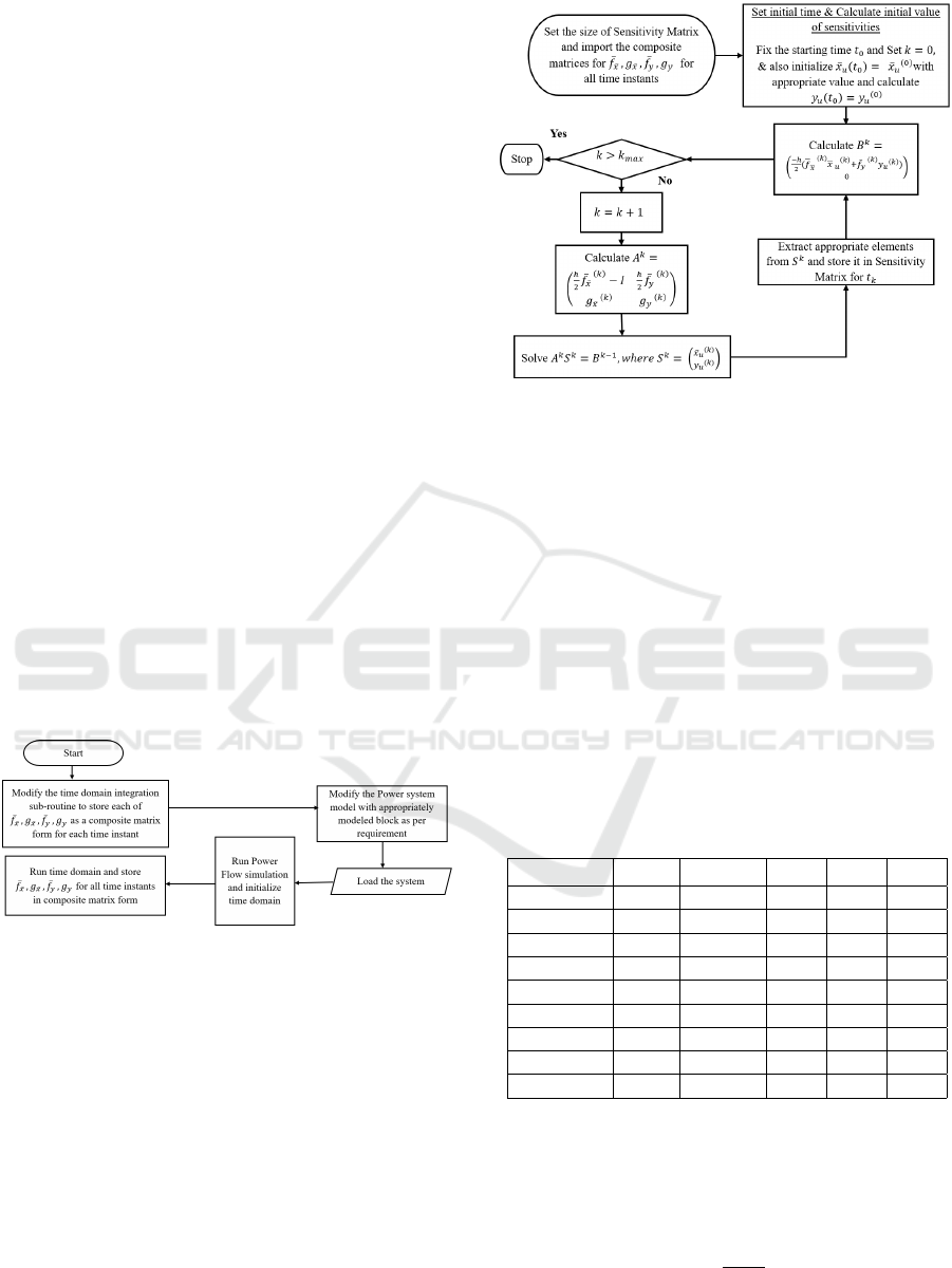
4 ARCHITECTURE OF

EXTENDED PSAT FOR

TRAJECTORY SENSITIVITIES

A proposed architecture for computing tarjectory sen-

sitivities with respect to control input is shown in

Figure 7 & 8; it consists of two blocks: the basic

PSAT algorithm (Block-1), and the Trajectory Sen-

sitivity Calculation block (Block-2). The PSAT al-

gorithm of Block-1 includes the power ﬂow solution

and the modiﬁed time domain integration subroutines

for controls-augmented states to yield

¯x

all sampling instants from which all the 6 Jacobians

are extracted. The Trajectory Sensitivity Calculation

block (Block-2) then imports all the required elements

from Block-1 and computes and stores the trajec-

tory sensitivity values ¯x

, y

for each sampling instant

from which x

and y

can further be extracted.

Figure 7: Block-1.

4.1 PSAT Implementation & Validation

For validation, the same 9-bus 3-generator WECC test

system shown in Figure 3, with 3 appropriately mod-

eled SVC blocks at bus 5, bus 7, and bus 8 is selected.

These are designated as control-1 (u

), control-2 (u

control-3 (u

). The entire system is simulated in

PSAT and for each sampling instant, the trajectory

sensitivities of bus voltages with respect to u

, u

, and

are computed, using the algorithm mentioned in

the previous section.

Letting S

n j

denote the trajectory sensitivity of nth

bus voltage at its nominal value, V

, with respect the

jth control input as, u

, when the jth control input is

Figure 8: Block-2.

changed by ∆u

amount, the resulting voltage

the nth bus can be approximated by,

= V

∑

n j

∆u

(29)

In the simulation of the nominal system, the con-

trol inputs are chosen as, u

= 0 p.u., u

= 0 p.u., and

= 0 p.u. This system is simulated in PSAT and for

analysis purposes, the voltages of buses 4, 5, and 8, at

3 different sampling instants are tabulated in Table 1,

along with the corresponding trajectory sensitivities.

Using equation (29), the predicted voltages

are cal-

culated for the change in control inputs ∆u

= 0.01

p.u., ∆u

= 0.01 p.u., and ∆u

= 0.01 p.u. The values

are listed in Table 2.

Table 1: Simulation Results under Base Load.

Time-instant Bus no. V

(in p.u.) S

t = 1.15s Bus 4 0.9652 0.0248 0.0298 0.0334

t = 1.15s Bus 5 0.7098 0.1511 0.1150 0.0977

t = 1.15s Bus 8 0.8204 0.0755 0.0907 0.1014

t = 22.75s Bus 4 1.0172 0.0781 0.0718 0.0868

t = 22.75s Bus 5 0.8403 0.2233 0.1427 0.1355

t = 22.75s Bus 8 0.9426 0.1283 0.1208 0.1472

t = 40.05s Bus 4 0.9852 0.2437 0.2019 0.2210

t = 40.05s Bus 5 0.7781 0.5483 0.3987 0.3941

t = 40.05s Bus 8 0.8956 0.3861 0.3238 0.3533

To validate the estimated results, the system is

now simulated with u

= 0.01 p.u., u

= 0.01 p.u. &

= 0.01 p.u., while the simulated bus voltages V

are also depicted in Table 2. The percentage error of

simulated versus estimated values of bus voltages are

determined by %error =

−V

× 100. The last col-

umn of Table 2 shows the values of percentage errors

which are all well below 0.5%.

Computation of Trajectory Sensitivities with Respect to Control and Implementation in PSAT

757

Table 2: Percentage Error of Estimated results and Simu-

lated results for ∆u

= 0.01 p.u.,∆u

= 0.01 p.u. & ∆u

0.01 p.u.

Time instant Bus no.

(in p.u.)

(in p.u.) % error

t = 1.15s Bus 4 0.9661 0.9662 -0.0073

t = 1.15s Bus 5 0.7134 0.7131 0.0503

t = 1.15s Bus 8 0.8231 0.8229 0.0261

t = 22.75s Bus 4 1.0196 1.0197 -0.0007

t = 22.75s Bus 5 0.8454 0.8453 0.0017

t = 22.75s Bus 8 0.9466 0.9465 0.0012

t = 40.05s Bus 4 0.9918 0.9915 0.0341

t = 40.05s Bus 5 0.7916 0.7907 0.1025

t = 40.05s Bus 8 0.9063 0.9056 0.0691

In order to validate our approach of computing the

trajectory sensitivity with respect to loads as the con-

trol inputs, we designate the load at bus 6 as control-

4 (u

), where u

= P

+ jQ

. Now, keeping other

control inputs u

, u

and u

unchanged, for ∆u

∆P

+ j∆Q

= 0.01 + j0.01, the trajectory-sensitivity

based predicted versus the simulated voltages are ob-

tained using the process as described earlier in Ta-

ble 3, followed by the calculation of percentage er-

rors, which was found to less than 0.5% (see Table 4).

Note in Table 3, in accordance to the previous nota-

tion, S

n j

& S

n j

, represents trajectory sensitivity of nth

bus with respect to base active power (P

) and base

reactive power (Q

) of the jth load.

Table 3: Simulation Results under Base Load.

Time-instant Bus no. V

(in p.u.) S

t = 8.50s Bus 4 1.0222 -0.0729 -0.0625

t = 8.50s Bus 5 0.89336 -0.0514 -0.0405

t = 8.50s Bus 8 0.96806 -0.0576 -0.0480

t = 28.00s Bus 4 1.0089 -0.1348 -0.0888

t = 28.00s Bus 5 0.86050 -0.1051 -0.0665

t = 28.00s Bus 8 0.94473 -0.1084 -0.07099

t = 38.60s Bus 4 0.99538 -0.1877 -0.1144

t = 38.60s Bus 5 0.83686 -0.1782 -0.1068

t = 38.60s Bus 8 0.92645 -0.1718 -0.1051

These results validate the proposed method of

computation of trajectory sensitivities with respect

to the control inputs as proposed by our control-

augmented state-space method, numerical integra-

tion, and their PSAT implementation.

4.2 A Speciﬁc Application of the

Implementation

The proposed implementation extends the functional-

ity of the software PSAT for computation trajectory

Table 4: Percentage Error of Estimated versus Simulated

results for ∆u

= 0.01 + j0.01 with ∆u

= ∆u

= 0.

Time instant Bus no.

(in p.u.) V

(in p.u.) % error

t = 8.50s Bus 4 1.0235 1.02276 0.0797

t = 8.50s Bus 5 0.89428 0.89364 0.07134

t = 8.50s Bus 8 0.96912 0.96839 0.0755

t = 28.00s Bus 4 1.0112 1.0096 0.1545

t = 28.00s Bus 5 0.86222 0.8608 0.1602

t = 28.00s Bus 8 0.94652 0.94511 0.1498

t = 38.60s Bus 4 0.99841 0.99619 0.2219

t = 38.60s Bus 5 0.83971 0.83735 0.2810

t = 38.60s Bus 8 0.92922 0.92697 0.2427

sensitivities with respect to any control inputs and pa-

rameters other than the system variables, enhancing

the PSAT’s capabilities beyond simulation, to control

synthesis.

As an example, in Model Predictive based con-

troller based voltage stability scheme, the common

control actions are switching of shunt capacitors, rais-

ing/lowering of Under load tap-changers, and exer-

cising load-shedding in a coordinated manner. The

corresponding optimization problem is complex in

case of large power system comprising of highly non-

linear component dynamics. In this context, the com-

putation of voltage trajectory sensitivities with respect

to control inputs provides an efﬁcient way to estimate

the effect of control inputs on voltage trajectories, and

selecting an optimal control strategy.

As discussed earlier, in the available version of

PSAT, there is no speciﬁc sub-routine to calculate

trajectory sensitivity with respect to control inputs.

Further such computation also requires the computa-

tion of the Jacobian matrices with respect to controls,

which are also not made available in PSAT. Our im-

plementation extends PSAT to facilitate the computa-

tion of such Jacobians with respect to control inputs

as well as parameterized loads by augmenting the re-

spective control inputs and load parameters into the

state variables, with zero dynamics. This not only

helps to compute trajectory sensitivities with respect

to controls, but also enables the computation of load

margin sensitivity, and study of neighbouring trajec-

tories under different control actions or variation of

parameters.

5 CONCLUSION

This paper presented a way of computing trajectory

sensitivity with respect to control in PSAT based

on augmentation of state-space with zero-dynamics

controls. Three types of control were considered:

ICINCO 2019 - 16th International Conference on Informatics in Control, Automation and Robotics

758

SVC, ULTC, and Loads. With proper modiﬁcation

of certain parameters of available control models in

PSAT, it became possible to achieve the desired zero-

dynamics of control, and then to calculate the desired

trajectory sensitivities. Our approach thus enables a

convenient way for designing of real-time protection

schemes, such as MPC, that use trajectory sensitives

to quickly estimate future behaviors due to changes in

inputs and initial state/algebraic variables. The paper

also described the structure of the algorithm for com-

puting trajectory sensitivities, and presented the vali-

dation of the trajectory sensitivity computation results

by computing the same values through direct simula-

tions of trajectories under various control inputs. The

percentage error was found to be no more than 0.5%.

The extended PSAT implementation is further be-

ing developed for model-predictive control applica-

tion.

ACKNOWLEDGEMENTS

The work was supported in part by the Na-

tional Science Foundation under the grants, NSF-

CCF-1331390, NSF-ECCS-1509420, and NSF-IIP-

1602089.

REFERENCES

Abdelsalam, H. A., Suriyamongkol, D., and Makram, E. B.

(2017). A tsa-based consideration to design lqr auxil-

iary voltage control of dﬁg. In 2017 North American

Power Symposium (NAPS), pages 1–6. IEEE.

Chatterjee, D. and Ghosh, A. (2007). Transient stability

assessment of power systems containing series and

shunt compensators. IEEE Transactions on Power

Systems, 22(3):1210–1220.

Ferreira, C. M., Pinto, J. D., and Barbosa, F. M. (2004).

Transient stability assessment of an electric power

system using trajectory sensitivity analysis. In 39th

International Universities Power Engineering Con-

ference, 2004. UPEC 2004., volume 3, pages 1091–

1095. IEEE.

Ghosh, A., Chatterjee, D., Bhandiwad, P., and Pai, M.

(2004). Trajectory sensitivity analysis of tcsc com-

pensated power systems. In IEEE Power Engineering

Society General Meeting, 2004., pages 1515–1520.

IEEE.

Hiskens, I. and Gong, B. (2005). Mpc-based load shedding

for voltage stability enhancement. In Proceedings of

the 44th IEEE Conference on Decision and Control,

pages 4463–4468. IEEE.

Hiskens, I. A. and Pai, M. (2000). Trajectory sensitivity

analysis of hybrid systems. IEEE Transactions on Cir-

cuits and Systems I: Fundamental Theory and Appli-

cations, 47(2):204–220.

Hiskens, I. A. and Pai, M. (2002). Power system ap-

plications of trajectory sensitivities. In 2002 IEEE

Power Engineering Society Winter Meeting. Confer-

ence Proceedings (Cat. No. 02CH37309), volume 2,

pages 1200–1205. IEEE.

Jin, L., Kumar, R., and Elia, N. (2007). Application

of model predictive control in voltage stabilization.

In 2007 American Control Conference, pages 5916–

5921. IEEE.

Jin, L., Kumar, R., and Elia, N. (2010). Model pre-

dictive control-based real-time power system protec-

tion schemes. IEEE Transactions on Power Systems,

25(2):988–998.

Laufenberg, M. J. and Pai, M. (1997). A new approach to

dynamic security assessment using trajectory sensitiv-

ities. In Proceedings of the 20th International Confer-

ence on Power Industry Computer Applications, pages

272–277. IEEE.

Milano, F. (2005). An open source power system analy-

sis toolbox. IEEE Transactions on Power systems,

20(3):1199–1206.

Milano, F. (2011). Hybrid control model of under load

tap changers. IEEE Transactions on Power Delivery,

26(4):2837–2844.

Milano, F., Vanfretti, L., and Morataya, J. C. (2008). An

open source power system virtual laboratory: The psat

case and experience. IEEE Transactions on Educa-

tion, 51(1):17–23.

Nasri, A., Eriksson, R., and Ghandhari, M. (2013a). Suit-

able placements of multiple facts devices to improve

the transient stability using trajectory sensitivity anal-

ysis. In 2013 North American Power Symposium

(NAPS), pages 1–6. IEEE.

Nasri, A., Eriksson, R., and Ghandhari, M. (2014). Using

trajectory sensitivity analysis to ﬁnd suitable locations

of series compensators for improving rotor angle sta-

bility. Electric Power Systems Research, 111:1–8.

Nasri, A., Ghandhari, M., and Eriksson, R. (2013b). Tran-

sient stability assessment of power systems in the

presence of shunt compensators using trajectory sensi-

tivity analysis. In 2013 IEEE Power & Energy Society

General Meeting, pages 1–5. IEEE.

Tang, L. and McCalley, J. (2013). Trajectory sensitivities:

Applications in power systems and estimation accu-

racy reﬁnement. In 2013 IEEE Power & Energy Soci-

ety General Meeting, pages 1–5. IEEE.

Zima, M. and Andersson, G. (2003). Stability assessment

and emergency control method using trajectory sensi-

tivities. In 2003 IEEE Bologna Power Tech Confer-

ence Proceedings,, volume 2, pages 7–pp. IEEE.

Computation of Trajectory Sensitivities with Respect to Control and Implementation in PSAT

759