
Optimal Waypoint Navigation for Underactuated Cruising AUVs
Kangsoo Kim
National Maritime Research Institute, National Institute of Maritime, Port, and Aviation Technology, 6-38-1 Shinkawa,
Mitaka, Tokyo 181-0004, Japan
Keywords: Navigation, Waypoint, Optimization, Depth, Altitude, Cruising AUV, Bottom Collision.
Abstract: An advanced approach to the waypoint-based navigation for near-bottom survey of a cruising AUV is
presented. Pursuing vehicle safety as well as high-definition bottom survey data, we apply GDS-based
optimization technique for achieving waypoint-based minimum-altitude flight of an underactuated cruising
AUV. While the objective of our optimization is minimizing average altitude of a vehicle throughout its flight
interval, depth or altitude references on waypoints are used as control inputs. In our optimization, bottom
bathymetry is incorporated as a constraint used for bottom collision avoidance. As another constraint, dynamic
model of an AUV is included. By solving the dynamic model in time domain, motion responses of the vehicle
following reference waypoints are derived. Our approach of the optimal waypoint navigation is validated by
not only simulation but also at-sea deployment of an AUV.
1 INTRODUCTION
Providing far higher resolution bottom survey data
than can be obtained from surface vessels, AUVs are
increasingly being used in a diverse range of
applications in the scientific, military, commercial,
and policy sectors (Wynn et al., 2014). However, as
its altitude from the bottom decreases, an AUV is
faced with higher risk of bottom collision. The risk of
bottom collision is especially serious when an
underactuated vehicle exercises low-altitude flight
over a steep and rugged terrain. It is common to
classify AUVs into two categories according to their
behavioral character: hovering and cruising (McPhail
et al., 2010). It can be said that cruising AUVs are
typically the choice for higher-speed, longer-range
missions. In general, a hovering AUV can hover and
maneuver around an operating point, while most
cruising AUVs cannot. This is because most cruising
AUVs are underactuated, and thus have restricted
path-following capability (Lea et al., 1999). Due to
this restriction, a cruising AUV has difficulty in
avoiding impending collision with the obstacles in
close proximity, which discourages it from flying
over a steep and rugged terrain. Another concern of
the flight of a cruising AUV over a steep and rugged
terrain is that its onboard sonar altimeter is
susceptible to so called "loss of bottom lock". Once
occurs, the loss of bottom lock disables the use of
correct vehicle altitude, leading to the increased
hazard of bottom collision (Keranen et al., 2012). In
this paper, we demonstrate that the loss of bottom
lock is especially favored by a bottom-following
flight over a steep and rugged terrain. Unlike altitude,
the depth of an underwater vehicle is highly accurate
and reliable, being obtainable merely by measuring
ambient water pressure. In this paper, we present
depth-based optimal waypoint navigation as an
alternative for the altitude-based acoustic navigation.
By following the waypoints derived by GDS
(gradient descent search)-based optimization, an
AUV achieves minimum-altitude flight over a steep
and rugged terrain avoiding bottom collision.
2 WAYPOINT NAVIGATION
In underwater vehicle navigation, waypoints are the
set of 3D coordinates identifying the navigational
points defined as the latitude, longitude, and depth or
altitude pairs. Within the framework of waypoint
navigation, a vehicle moves toward a destination
passing through the reference waypoints. Figure 1
shows a sample of waypoints generated for AUV-
based near-bottom survey of a submarine volcano. As
shown, the reference path is spontaneously defined by
the waypoints. In Fig. 1, it is noted that the numbers
attached to each waypoint represent reference depths.
124
Kim, K.
Optimal Waypoint Navigation for Underactuated Cruising AUVS.
DOI: 10.5220/0007931901240134
In Proceedings of the 16th International Conference on Informatics in Control, Automation and Robotics (ICINCO 2019), pages 124-134
ISBN: 978-989-758-380-3
Copyright
c
2019 by SCITEPRESS – Science and Technology Publications, Lda. All rights reserved
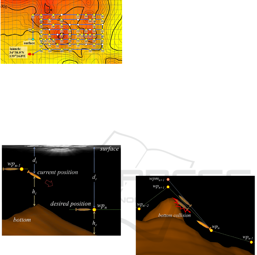
Figure 1: Waypoints and reference path generated for a
near-bottom survey by an AUV.
In our waypoint-based navigation, the reference depth
of n-th waypoint, (i.e. wp
n
) shown in Fig. 1 is the
desired depth to be reached by a vehicle during its
transit between wp
n-1
and wp
n
. Therefore, no sooner
has the vehicle arrived at wp
n-1
, its target vertical
position is updated to the reference depth of wp
n
(Fig.
2). In Fig. 2, d
i
and d
r
are the current and the desired
(reference) vehicle depths, while h
i
and h
r
are their
altitude counterparts, respectively.
Figure 2: Waypoint-based depth control of an AUV.
It is to be noted here that instead of depth, altitude
from the bottom also can be used for controlling the
vertical position of an underwater vehicle. In our
work, altitude means the absolute altitude in air
navigation, i.e., the height of a vehicle above the
terrain over which it is traversing (U.S. Air Force,
2005). The altitude control works on the basis of the
altitude error e
h
defined as the difference between the
reference and the current altitude of a vehicle. It is
noted that, however, by substituting the altitude error
with its depth error counterpart, a depth controller is
also able to exercise the altitude control equivalently.
Hence, it is very common that a depth controller of an
AUV is also in charge of the altitude control (McPhail
et al., 2010; Kim and Ura, 2015). In such cases, we
can recognize that for the altitude control
e
d
= -e
h
(1)
where e
d
is the depth error counterpart of the current
vehicle altitude error e
h
= h
r
- h
i
.
3 NEAR-BOTTOM SURVEY
FLIGHT
Near-bottom survey of a seafloor is one of the most
important AUV missions in its diverse applications.
Being able to fly close to the bottom, AUVs are
capable of collecting seafloor mapping, profiling and
imaging data of far higher resolution and navigational
accuracy than surface vessels (Wynn et al., 2014).
However, moving close to the bottom inevitably
raises the risk of bottom collision. This is especially
serious when a cruising AUV is flying over a rugged
and steep terrain keeping low altitude above the
bottom.
3.1 Bottom Collision
Figure 3 illustrates the possible bottom collision of a
cruising AUV during its waypoint-based near-bottom
mission over a steep and rugged terrain.
Figure 3: Bottom collision of an underactuated cruising
AUV over steep and rugged terrain.
Suppose that the reference depth of any waypoint is
merely assigned as the depth determined by an
arbitrary constant altitude above the bottom. Then,
although the reference path generated by interlinking
adjacent waypoints runs over the seafloor without any
interference with the terrain, an underactuated vehicle
following the waypoints can cause a bottom collision
(Fig. 3). This is because the reference path has been
generated without considering the constraint of
vehicle dynamics which can let the vehicle faced with
too low altitude to avoid imminent bottom collision.
In Fig. 3, bottom collision occurs within the path
Optimal Waypoint Navigation for Underactuated Cruising AUVS
125
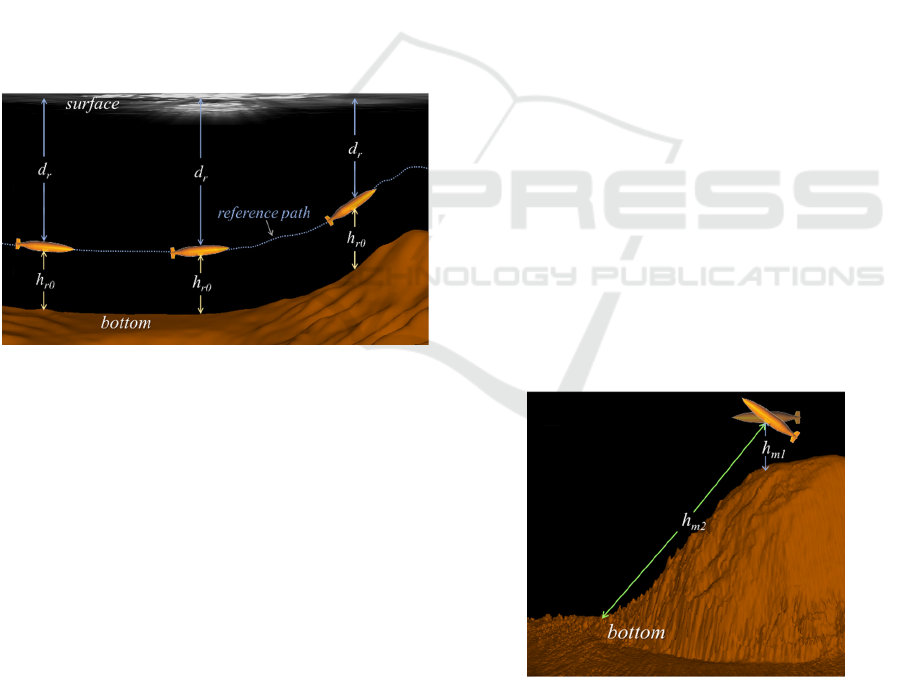
interval between [wp
n
~ wp
n+1
]. However, by
modifying the reference depths of the waypoints
within the interval, i.e., by substituting wpm
n+1
for
wp
n+1
, for example, we can make the vehicle avoid
bottom collision, as shown in the figure. As can be
noticed from Fig. 3, in order to avoid bottom collision,
the constraint of vehicle dynamics as well as the
bottom topography should be considered.
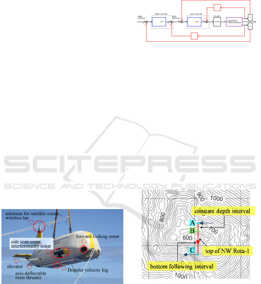
3.2 Bottom-following Flight
As mentioned previously, altitude can be used in
determining the vertical reference position of a
vehicle. A typical example of such approach is the
navigation so called bottom following (Caccia et al.,
2003). In the bottom-following flight, a vehicle is
controlled to follow the bottom maintaining a fixed
altitude above it (Fig. 4). Thus, a device for
measuring current vehicle altitude is essential for
practicing a bottom-following flight. Most modern
AUVs are equipped with a bottom-lock sonar such as
DVL (Doppler Velocity Log) for this purpose.
Figure 4: Bottom-following flight of a cruising AUV.
In Fig. 4, h
r0
is the constant reference altitude
assigned for a bottom-following flight. It is noted that
while h
r0
is constant, d
r
changes according to current
vehicle position. When the bottom-following flight
works without fail, a vehicle exactly follows the
reference path defined as the along-track bottom
section parallelly shifted upward by h
r0
(Fig. 4). In
practice, however, the bottom following is not so
reliable as the waypoint-based depth control because
it relies entirely on real-time vehicle altitudes
provided by a bottom-lock sonar.
4 ACOUSTIC NAVIGATION
In general, depth sensor installed in most modern
AUVs is a quartz crystal pressure sensor calculating
current vehicle depth from the direct measurement of
ambient seawater pressure. It is known that such
pressure sensor provides very high precision whose
accuracy of 0.01% of full scale (Kinsey et al., 2006).
Therefore, it is noted that waypoint-based depth
control is a highly reliable means for achieving stable
and robust underwater vehicle navigation in vertical
plane. As regards vehicle altitude, a bottom-lock
sonar working on the basis of the single range
acoustic time-of-flight navigation is used in
estimating its current value above the bottom.
Varying with the frequency of carrier signal,
precision of echo sounding is said to be 0.01 ~ 1.0 m
(Kinsey et al., 2006). The precision seems to be
acceptable for near-bottom flight of a cruising AUV.
However, there still is a serious concern in acoustic
time-of-flight navigation. Altitude measurement by
using a bottom-lock sonar system is highly vulnerable
to the surrounding environment.
4.1 Altitude Overestimation
The first vulnerability of the altitude-based bottom-
following flight of a cruising AUV is possible
overestimation of the vehicle altitude over a steep
terrain. As shown in Fig. 5, over a steep terrain, even
a small change in vehicle's attitude may result in a
large variation of indicated altitude. Suppose that a
vehicle following the bottom is instantaneously
taking large nose-up attitude when it has reached a
steep downhill. Then, indicated altitude h
m2
is used
for ongoing bottom-following flight instead of h
m1
,
the true altitude. Since h
m2
is largely overestimated
compared to its true counterpart, the vehicle may try
to approach the bottom further lowering its altitude
even when h
m1
is smaller than h
r0
.
Figure 5: Indicated and true altitudes over a steep terrain.
4.2 Loss of Bottom Lock
In order for a bottom-lock sonar system to work
properly, its receiver signal-to-noise ratio (SNR)
ICINCO 2019 - 16th International Conference on Informatics in Control, Automation and Robotics
126
should be higher than the detectable limit called
threshold SNR (Urick, 1982). Since the acoustic
energy projected by a transmitter dissipates due to the
transmission losses, echoes show markedly reduced
acoustic intensity from the source level (SL).
Moreover, when a travelling acoustic wave
encounters sea bottom leading to an echo event, some
fraction of its energy is transmitted into the bottom.
Dissipation in seawater and transmission into the sea
bottom of acoustic energy are the major sources of
reduced echo level (EL) lowering SNR (Urick, 1982).
When the EL of sonar echo is so small as for its SNR
to be lower than the threshold value, a bottom-lock
sonar is no longer able to lock on to the seafloor. This
state is called "loss of bottom lock" in which any
bottom-reference sonar observation is unavailable.
Losing the information of current altitude, an
underwater vehicle following a seafloor for near-
bottom flight is faced with the serious risk of bottom
collision when loss of bottom lock occurs.
5 MOTION INSTABILITIES
We experienced serious motion instabilities of a
cruising AUV during its mission of surveying a
submarine volcano called NW Rota-1. Figure 6
shows the AUV r2D4 having been deployed in NW
Rota-1 site. The r2D4 is a cruising AUV developed
by Institute of Industrial Science, the University of
Tokyo (Kim and Ura, 2009). NW Rota-1 is an active
submarine volcano, located in 64 km NW of the
island of Rota in the western Pacific Ocean.
Figure 6: Overall layout of r2D4.
5.1 Control and Navigation
Figure 7 shows the schematic block diagram of depth
control implemented in r2D4 (Kim and Ura, 2009). It
is noted here that the duality mentioned above is
applied to the depth and altitude control or r2D4. That
is, it is the depth controller shown in Fig. 8 that
actually works corresponding to the altitude control
exercised by bottom following.
Figure 7: Block diagram of the depth control of r2D4.
In Fig. 7, e
z
and e
are depth and pith errors;
r
and
are reference and output pitch; d is vehicle depth; q is
pitch rate; u and w are surge and heave velocities; and
el
and
Cel
are elevator deflection and its command,
respectively. K denotes controller gain while T
derivative or integral time.
Figure 8 shows the navigation applied to r2D4 during
its NW Rota-1 survey mission. In Fig. 8, AC is a part
of the reference path generated for r2D4 flight #16.
AC is called the "near-the-top" interval, generated for
covering the area in the vicinity of the top of NW
Rota-1. In flight #16, both constant depth flight and
bottom following were used as the navigation for
bottom survey. To the anterior section AB of the near-
the-top interval, constant depth flight with the
reference depth of 510 m was applied. Along the
posterior section BC, on the other hand, vehicle was
made to follow the bottom keeping its altitude 150 m
off the bottom.
Figure 8: Navigation applied to near-the-top path interval.
5.2 Motion Instabilities over a Steep
Terrain
Figure 9 shows the bottom cross section of NW Rota-
1 taken along the near-the-top interval. Bottom
bathymetry along a vehicle trajectory is obtained
merely by summing the vehicle depth and the altitude
(s
)
d
r
sT
1
1K-
iz
pz
dzpz
TK-
(s)
r
sT
1
1K
i
p
(s)e
z
(s)e
d
d
s
(s)
Cel
(s)
el
q(s)
w(s)
s
1
(s)
w(s)
d(s)
(s)
q(s)
dp
TK
d(s)
u(s)
s
1
Optimal Waypoint Navigation for Underactuated Cruising AUVS
127
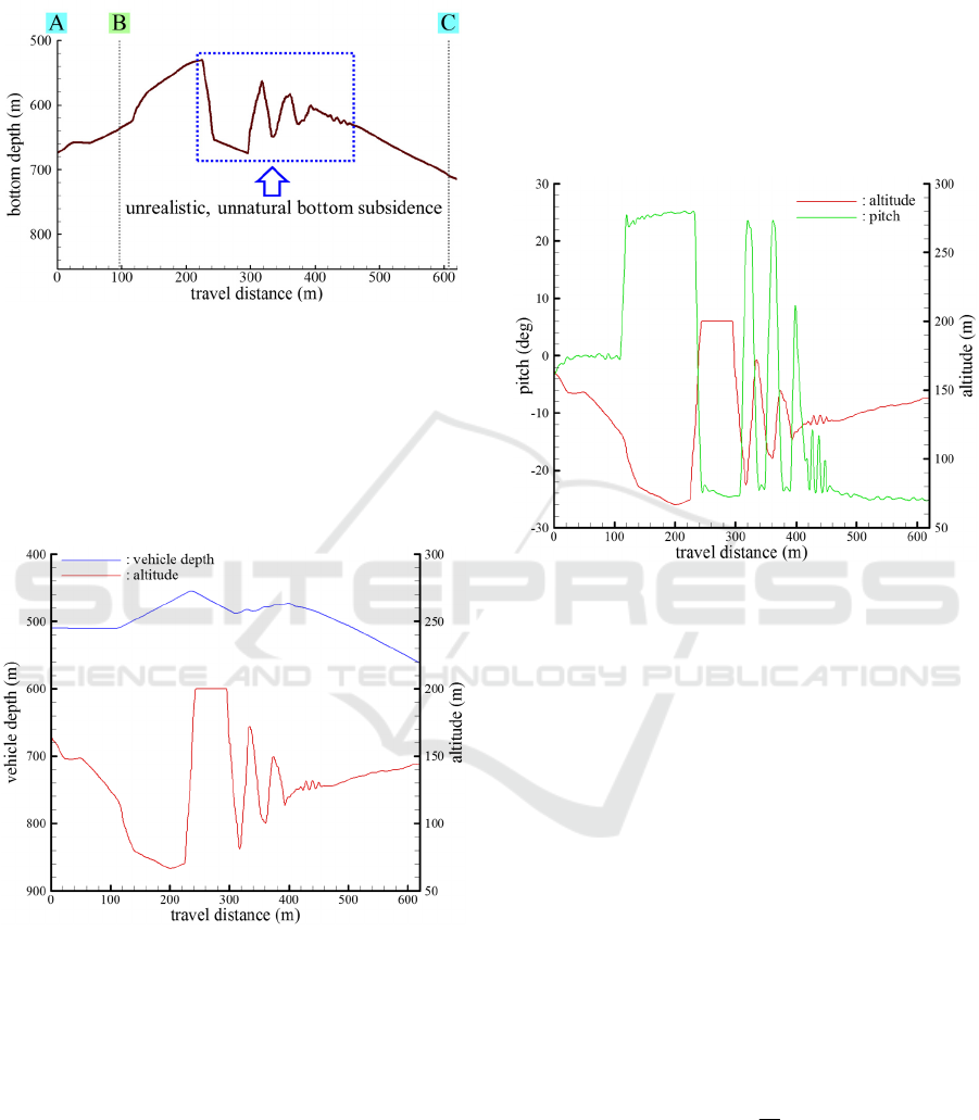
sequences. In the bottom cross section obtained, we
find saw-teeth like, large and unnatural subsidence
continuing along the descending terrain (Fig. 9).
Figure 9: Vertical cross section of submarine volcano NW
Rota-1 along near-the-top path interval.
Motivated by this too unrealistic shape of the bottom
cross section, we checked the time sequences of
vehicle's depth, altitude, and pitch taken from the log
of r2D4 flight #16. Figure 10 shows depth and
altitude sequences taken along the near-the-top path
interval shown in Figs. 8 and 9.
Figure 10: Vehicle depth and altitude.
In Fig. 10, we notice that while fluctuating slightly,
the depth sequence seems normal, since its rate of
change is reasonable within the normal range of the
heave rate of r2D4. On the other hand, however, the
altitude is definitely erroneous since the maximum
value of its time derivative reaches 13.8 m/s which is
more than 9 times the cruising speed of r2D4. Figure
11 shows pitch sequence of the vehicle together with
its altitude counterpart. As can be expected from
intrinsic heave-pitch coupling of a longitudinally
asymmetrical slender body, vehicle's pitch also
fluctuates synchronizing with the altitude fluctuation.
It is noted here that pitch fluctuates bounded within
the range of -25 to 25 which are the predefined
lower and upper limits of the pitch reference. Judging
from its magnitude as well as rate of change, pitch
does not show any notable abnormality.
Acknowledging that the measured vehicle depth is
normal, we can conclude that it is erroneous vehicle
altitude that is responsible for the unrealistic bottom
cross section obtained.
Figure 11: Pitch and altitude.
5.3 Acoustic Bottom Backscatter
If we apply the sonar equation (Urick, 1983; Morgan,
1978; Miline, 1983) to our DVL altimeter, the echo
level (EL) of returned signal is
EL = SL - 2TL +TS (2)
where SL, TL, TS are the source level, the
transmission loss, and the target strength, respectively.
If NL denotes the noise level, we obtain the receiver
SNR as follows.
SNR = EL - NL = SL - 2TL +TS – NL (3)
In (3), energy loss arising from bottom scattering is
expressed by means of the target strength (Morgan,
1978; Urick, 1983). In an active sonar, the target
strength is a measure of the reflecting power of a
sonar target defined as
(4)
where I
i
and I
s
are the incident and the scattered
acoustic intensities, respectively.
As the bottom is an effective reflector and scatterer of
sound, it acts to redistribute a portion of the sound in
i
s
10
I
I
10logTS
ICINCO 2019 - 16th International Conference on Informatics in Control, Automation and Robotics
128
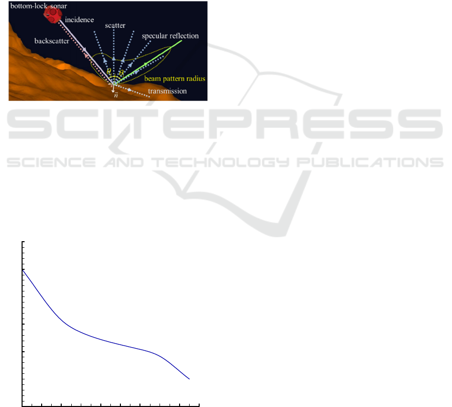
the ocean (Urick, 1983). Not all of the sound is
reflected or scattered, however, but some fraction of
acoustic energy is transmitted into the bottom. The
acoustic bottom backscatter is the reflection of sound
on a sea bottom back to the direction from which it
came (Fig. 12). Therefore, it is the backscattered
sound that primarily activates a bottom-lock sonar. In
case of acoustic bottom scatter, TS, the sonar target
strength is frequently referred to as bottom strength.
Also, it is well known that the bottom strength
directly depends on the incidence angle of impinging
acoustic ray. More precisely, providing the maximum
strength at normal incidence, i.e., zero incidence
angle, the bottom strength decreases notably as the
incidence angle increases (Urick, 1983; Moustier and
Alexandrou, 1991).
Figure 12: Sound redistribution on the bottom by the
impinging acoustic ray of incidence angle
i
.
It is well known that bottom strength is also
dependent on the sound frequency of impinging
acoustic ray (Mackenzie, 1961; Urick, 1983). In r2D4,
a 300 kHz, 4-beam DVL is used as altimeter. Li et al.
(2012) presents a smooth curve of 300 kHz bottom
acoustic backscatter as a function of incidence angle
(Fig. 13). By using the curve, we can easily evaluate
I
s
corresponding to any incidence angle on the bottom.
Figure 13: Bottom backscatter strength of 300 kHz sound.
It is officially announced that the source level and the
maximum range of our DVL are 216.3 dB and 200 m,
respectively (Teledyne RD Instruments, 2013). This
enables us to estimate the threshold SNR of our DVL
altimeter to be 35.7 dB (Kim and Ura, 2015).
Transmission loss in (2) and (3) can be calculated by
TL = TL
sp
+ TL
at
= 20log
10
R +
R
(5)
where TL
sp
and TL
at
are the spherical spreading and
the attenuation, respectively which are two major
components of the transmission loss experienced by
an acoustic signal travelling in a fluid medium
(Morgan, 1978; Urick, 1983; Miline, 1983). In (5), R
is the distance from the source and
is the
logarithmic absorption coefficient relating the signal
intensity to range (Urick, 1983).
For the noise level, we consider external background
noise only ignoring cross-sensor acoustic interference.
This is because in general, an AUV employs multiple
sonars of totally different operating frequencies
(Edward et al., 2007), and so does r2D4. It is noted
that at the frequencies over 50 kHz, thermal noise
begins to dominate the underwater background noise
(Urick, 1984). In evaluating the thermal noise level
denoted as NL
th
, we use the following relation
(Mellen, 1952)
NL
th
= -15 + 20 log
10
f (6)
where f is the frequency of interest in kHz.
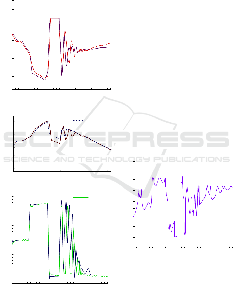
5.4 Simulated Bottom-following Flight
By using the mathematical model of underwater
acoustics given as (2) ~ (6) and the vehicle dynamics
of r2D4 (Kim and Ura, 2009), the near-bottom flight
of r2D4 following the path interval AC (Fig. 9) has
been simulated. All conditions of the simulation, e.g.,
the sea bottom topography, the flight path, and the
navigation were taken from the r2D4 flight #16
mentioned above. Figure 14 shows the time history of
simulated vehicle altitude. In Fig. 14, altitude log of
the actual flight is superposed on the simulated result.
As seen, like the actual flight, the simulation also
demonstrates severely fluctuating vehicle motion.
Moreover, as in the case with the actual flight, the
largest altitude peak comes first followed by the
gradually decaying smaller peaks. Figure 15 shows
the simulated vertical cross section of NW Rota-1
along the interval AC. The flight simulation generates
the same pattern of the bottom cross section as was
obtained from the actual flight. Simulated vehicle
pitch and the pitch log of the actual flight are shown
in Fig. 16. Over the whole, it is noted that the vehicle
incidence angle (deg)
bo
t
t
om bac
k
sca
t
t
e
r
s
t
r
eng
t
h(
d
B)
0 102030405060708090
-60
-50
-40
-30
-20
-10
0
Optimal Waypoint Navigation for Underactuated Cruising AUVS
129
behaviors and the along-track bottom bathymetry
obtained by the simulation show intrinsic similarities
to those taken from the actual flight.
Figure 14: Simulated and actual vehicle altitudes.
Figure 15: Simulated and actual bottom cross sections.
Figure 16: Simulated and actual vehicle pitch.
6 ALTERNATE NAVIGATION
6.1 Vulnerability of Acoustic
Navigation
In the previous section, bottom-following flight
simulation has reproduced the longitudinal motion
instabilities of a cruising AUV r2D4 having been
experienced during its actual near-bottom mission. In
the previous literature by the author, a probable
scenario explaining the generating mechanism of the
motion instabilities are presented (Kim and Ura,
2015). In this scenario, the loss of bottom lock of
DVL altimeter and the altitude overestimation are
identified as two major sources inducing instabilities
in longitudinal vehicle motion. Figure 18 shows the
receiver SNR of our 300 kHz DVL altimeter derived
from the flight simulation shown above. As already
mentioned, a bottom-lock sonar gets trapped into the
loss of bottom lock when the receiver SNR is lower
than its threshold. By comparing Fig. 15 to 17, we can
find that a sharp reduction in receiver SNR happens
when the vehicle is about to pass through the top of
NW Rota-1. And from Figs. 16 and 17, we notice that
the interval in which the receiver SNR drops below
its threshold nearly coincides with that of the first
peak of altitude fluctuation. Thus, it is natural to infer
that the large reduction in SNR is the direct source of
the first peak in altitude fluctuation.
Figure 17: Simulated receiver SNR of DVL altimeter.
The reason of the sharp reduction in receiver SNR can
be explained by the abrupt increase in acoustic
incidence angle on the bottom near the top of the
mountain. In order to follow an ascending terrain, a
cruising AUV has to get nose-up. For a bottom-lock
travel distance (m)
al
t
i
t
u
d
e(m)
0 100 200 300 400 500 600
40
80
120
160
200
240
: simulation
:ac
t
ual
f
ligh
t
t
r
avel distance
(
m
)
bottom
d
epth (m)
0 100 200 300 400 500 600
500
600
700
800
: simulation
: actual flight
travel distance (m)
pi
t
ch (deg)
0 100 200 300 400 500 600
-30
-20
-10
0
10
20
30
:simulation
: actual flight
travel distance (m)
r
eceive
r
SNR (
d
B)
0 100 200 300 400 500 600
20
30
40
50
60
70
threshold SNR (35.7 dB)
ICINCO 2019 - 16th International Conference on Informatics in Control, Automation and Robotics
130
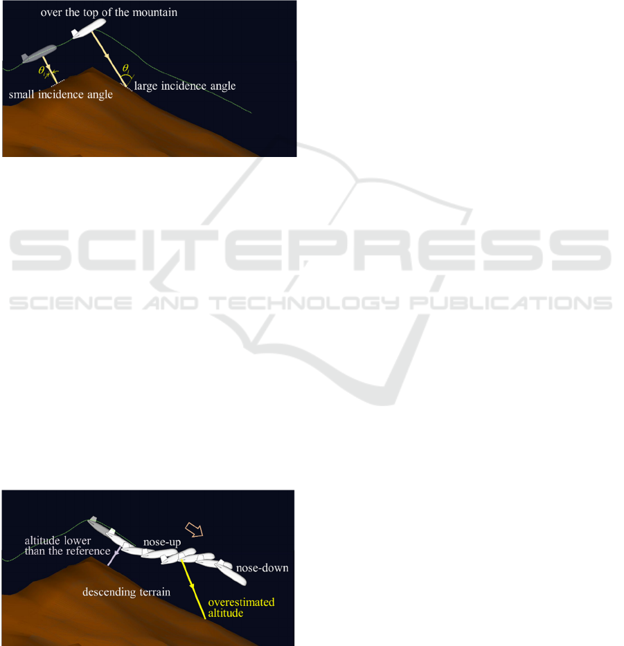
sonar, nose-up over an ascending terrain forms a
favorable operating condition, making incidence
angle small. Approaching the top of the mountain
with nose-up, however, makes the insonification
switched to descending terrain which leads to abrupt
increase in acoustic incidence angle (Fig. 18). Since
backscattered bottom strength weakens remarkably
as the bottom incidence angle increases (Fig. 13),
switched insonified area is thought to be the cause of
the sharp drop in receiver SNR, and eventually the
loss of bottom lock.
Figure 18: Switched insonified area.
Although the generation of the first altitude peak can
be well explained by the sudden drop of receiver SNR,
others cannot. In Fig. 17, we see whereas the altitude
continues to fluctuate, there is only one significant
SNR drop after 300 m of travel distance. As the
reason that r2D4 continued nodding motion even after
the extinction of significant SNR drop, we take notice
of the large variation in measured altitude over a steep
terrain. After recovering from the loss of bottom lock,
r2D4 pitches nose up over steep descent, resulting in
altitude overestimation. Once a cruising AUV gets a
largely overestimated altitude, it unduly pitches nose
down, in turn, in order to reduce the exaggerated
altitude immediately. In our scenario, the repeated
nose ups and nose downs, i.e., the nodding motion, of
excessive magnitude triggered by the loss of bottom
lock is the substance of motion instabilities appearing
irrespective of the SNR drop (Fig. 19).
Figure 19: Repetitive nodding motion of a cruising AUV
due to altitude overestimation.
6.2 Depth-based Navigation
As noticed from the simulation results shown above,
altitude-based acoustic navigation for a cruising AUV
has serious vulnerability to uneven bottom of steep
slope. When the motion instabilities explained so far
are detected during a near-bottom flight, it indicates
that the vehicle is currently exposed to a significant
hazard, since the occurrence of motion instabilities
implies that the vehicle is blind to its true altitude.
Furthermore, if the reference altitude is particularly
low, e.g., below tens of meters, the motion
instabilities put the vehicle at higher risk of bottom
collision. Therefore, in order to circumvent the risk of
bottom collision, more sophisticated navigation
strategy for near-bottom flight is required.
As already mentioned, the measured depth of an
underwater vehicle is far more reliable and accurate
compared to the measured altitude. Therefore, being
fundamentally free from the vulnerability to uneven
and steep terrain, depth-based navigation ensures
stable vehicle motion. Most depth-based navigation is
put into practice by means of waypoints. Controlling
actual vehicle trajectory, in practice, determining
reference depths on waypoints is highly important for
waypoint-based navigation. It is not easy, however,
for us to derive the reference waypoint depth which
produces the best performance in carrying out an
assigned mission.
6.3 Waypoints for Minimum Altitude
The definition of optimal waypoints differs according
to individual AUV flight missions. At present, it is
widely accepted that high-resolution bottom survey is
one of the most important and anticipative
expectations for AUV flight missions (Wynn et al.,
2013). In fact, the author's institute, National
Maritime Research Institute (NMRI) of Japan also
developed four cruising AUVs for high-resolution
survey of submarine hydrothermal sites (Kim and
Tamura, 2016). Considering these, we regard high-
resolution bottom survey as the major mission of our
AUV applications. Pursuing high-resolution bottom
survey, an AUV has to travel in as close proximity to
terrain as possible. Therefore, our optimal waypoints
are defined as those accomplishes the minimum-
altitude flight of an AUV. Figure 20 describes the
basic concept of our approach. By following the
optimal waypoints, an AUV conducts a near-bottom
flight minimizing the average altitude along its flight
path. In Fig. 20, h
a
is the minimum allowable altitude
within the flight path interval. It is noted here that h
a
Optimal Waypoint Navigation for Underactuated Cruising AUVS
131
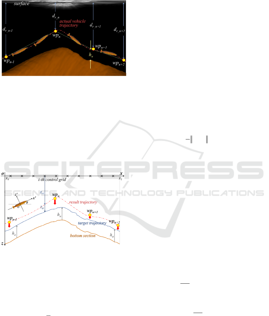
should be identical to the lowest (i.e., minimum)
altitude actually marked within the interval.
Figure 20: Minimum-altitude flight accomplished by
following optimal waypoints.
6.4 Problem Formulation
To treat the problem of optimal waypoint navigation,
two sets of coordinate system are employed: the
inertial (earth-fixed) coordinate system o-xz and the
body-fixed coordinate system o-x'z' (Fig. 21). While
waypoint optimization is carried out with respect to
the inertial frame, the motion response of a vehicle is
calculated using the equation of motion defined with
respect to the body-fixed frame.
Figure 21: Coordinate systems and schematic description of
the optimal waypoint derivation.
As already mentioned, the objective of our optimal
waypoint navigation problem is to derive the
waypoint set that minimizes average vehicle altitude
along a given flight path. Therefore, the performance
index of the problem is
(7a)
subject to
h(x) h
a
for x
[x
0
, x
1
]
(7b)
where h(x) is the vehicle altitude at a specified along-
track position x. In (7b), x
0
and x
1
are the along-track
coordinates of the lower and the upper limits of the
flight path interval of interest, and h
a
is the minimum
allowable altitude. It is obvious that once the
minimum allowable altitude h
a
is given, the ideal
behavior of a vehicle is to follow the bottom
throughout with its altitude of h
a
. Hence, the target
trajectory for optimizing the waypoints are given as
the envelope line of the bottom section shifted
upward (i.e., in -z direction) by h
a
, as shown in Fig.
21. In consequence, our problem results in the
optimization making the deviation between the target
and the result trajectories as small as possible. Let us
introduce so called "control grid" represented by the
cross symbol in Fig. 21. The control grid is a set of
arbitrarily spaced discrete points on x-axis at which
the deviation between the target and the result
trajectories is evaluated. Accordingly, by using the
control grid the performance index (7a) can be
redefined as
(8)
where z
t
and z
v
are the downrange position vectors of
the target trajectory and the vehicle defined at control
grids. Note that in this paper, variables in boldface
type denote vector or matrix. As already mentioned,
we use a GDS-based solution algorithm in
minimizing the performance index J in (8). In
deriving the solution, our algorithm works in an
iterative manner (Kim et al., 2011). By applying the
algorithm, the downrange position vector of the
waypoints is updated as
(9)
where z
w
i
is the downrange position vector of the
waypoints at i-th iteration step, estimated by adding
z
w
to z
w
i-1
. In (9), z
w
is the correction amount of z
w
computed by
(10a)
where
(10b)
In (10a),
is the gain and
is the non-physical
variable for the fictitious dimension of iteration. It is
noted that G is the Jacobian matrix of z
v
with respect
to the input vector z
w
.
1
0
x
x
2
(x)dxh
2
1
J
2
vt
-
2
1
J zz
w
1-i
w
i
w
zzz
T
tv
w
w
G--
d
d
zz
z
z
w
v
d
d
G
z
z
ICINCO 2019 - 16th International Conference on Informatics in Control, Automation and Robotics
132
7 RESULTS
The efficacy of waypoint-based minimum-altitude
navigation was validated through an actual near-
bottom survey mission using an AUV. In 2018, we
deployed an AUV called C-AUV#04 (Fig. 22) in a
potential hydrothermal vent site located in western
Pacific Ocean near Japan. C-AUV#04 is a high
maneuverability cruising AUV developed by NMRI
of Japan, having controllable pitch range of 80
(Kim et al., 2019). C-AUV#04 controls its flight
attitude by deflecting four movable fins mounted on
the stern (Fig. 22). It is noted that two horizontal fins
function as elevator and ailerons, while two vertical
fins as rudder. As for the depth or altitude control, C-
AUV#04 shares the same scheme of r2D4 explained
in section 5.1.
Figure 22: Overall layout of C-AUV#04.
When planning the path for C-AUV#04 flight #02
conducted for the near-bottom survey of the site, we
derived optimal reference depths for the waypoints
constituting the path interval covering western slope
of a sea mound. Figure 23 shows the waypoints with
their path interval superimposed on the bathymetric
map of the site. As seen, fourteen waypoints are to be
optimized in order to accomplish a depth-based,
minimum-altitude flight along the path.
Figure 23: Waypoints and path interval.
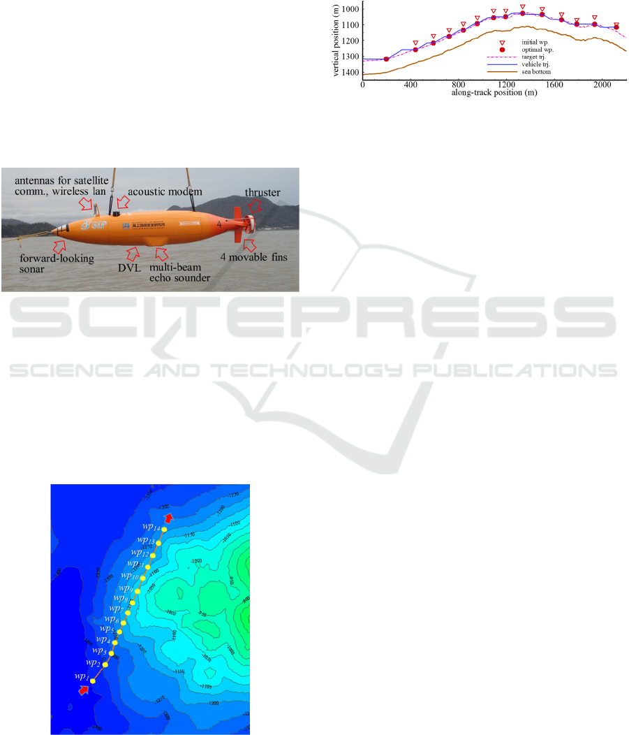
The results of near-bottom survey flight following
optimal waypoints are shown in Fig. 24. In
optimizing the waypoints, we assigned the initial
values of their reference depths with the water depths
at the points 120 m above the bottom (Fig. 24). And
it is also noted that the minimum allowable altitude is
set to 80 m.
Figure 24: Results of minimum-altitude flight.
By modifying the waypoints, the GDS-based solution
algorithm shifts the result trajectory away from the
initial waypoints lowering vehicle altitudes within the
flight path interval. Once a vehicle altitude derived by
the flight simulation reduces to around the minimum
allowable altitude, our algorithm terminates waypoint
modification and outputs current waypoint set as the
optimal solution. In this example, we can see small
overshoots in descending intervals, but the vehicle
successfully approaches the target trajectory, as a
whole (Fig. 24). Since they are quite close to the
minimum allowable altitude, the minimum altitudes
let the solution algorithm terminate waypoint
modification and take current waypoints as the
optimal waypoints for the minimum-altitude flight.
Uploaded to onboard storage device, derived optimal
waypoints are used for the near-bottom survey
mission. As can be seen in Fig. 24, by following the
optimal waypoint set derived by our simulation-based
approach, C-AUV#04 is able to complete near-
bottom survey mission successfully.
8 CONCLUSIONS
A systematic procedure for deriving optimal
waypoints used for AUV navigation has been
presented. Using GDS-based optimization, the
procedure derives optimal waypoints by following
which an underactuated cruising AUV accomplishes
minimum-altitude flight avoiding bottom collision.
Being a depth-based approach, the optimal waypoint
navigation is highly robust and fundamentally free
from the vulnerability of acoustic navigation. It is a
pregenerative approach, however, that requires the
real time revision of optimal waypoints in case the
vehicle is largely deviated from the planned path.
Optimal Waypoint Navigation for Underactuated Cruising AUVS
133

ACKNOWLEDGEMENTS
This work is partly supported by Council for Science,
Technology and Innovation (CSTI), cross-ministerial
Strategic Innovation Promotion Program (SIP), next-
generation technology for ocean resources
exploration (lead agency: JAMSTEC). Also, the
author would like to express special thanks to Japan
Marine Surveys Association (JAMSA) and Mr.
Takumi Sato of National Maritime Research Institute
(NMRI) of Japan, for their supports in AUV
operation.
REFERENCES
Wynn, B., Russel et al. (2014). Autonomous Underwater
Vehicles (AUVs): Their past, present and future
contributions to the advancement of marine geoscience.
Marine Geology, 352 (2014), 451–468.
McPhail, S., Furlong, M., and Pebody, M. (2010). Low-
altitude terrain following and collision avoidance in a
flight-class autonomous underwater vehicle.
Journal of
Engineering for the Maritime Environment
, 224 (4),
279–292
Lea, R. K., Allen R., and Merry S. L. (1999). A comparative
study of control techniques for an underwater flight
vehicle.
International Journal of System Science, 30 (9),
947–964.
Keranen, J. et al., (2012). Remotely-operated vehicle
applications in port and harbor site characterization:
Payloads, platforms, sensors, and operations.
Proc. of
IEEE Oceans 2012 Hampton Roads
.
U.S. Air Force (2005).
Air navigation. University Press of
the Pacific, Honolulu, ISBN 978-1410222466.
Kim, K. and Ura, T. (2015). Longitudinal motion instability
of a cruising AUV flying over a steep terrain,
IFAC-
PapersOnline
, vol.48, issue 2, 56–63.
Caccia, M., Bruzzone, G., Veruggio, G. (2003). Bottom-
following for remotely operated vehicles: Algorithms
and experiments.
Autonomous Robots, 14, 17–32.
Kinsey, J.C., Eustice, R.M., Whitcomb, L.L. (2006). A
survey of underwater vehicle navigation: Recent
advances and new challenges.
Proc. of 7th IFAC
Conference on Manoeuvring and Control of Marine
Craft
.
Urick, R.J. (1983).
Principles of underwater sound (3rd
edition)
. McGraw-Hill, New-York, ISBN 0-07-
066087-5.
Kim, K., and Ura, T. (2009). Optimal guidance for
autonomous underwater vehicle navigation within
undersea areas of current disturbance.
Advanced
Robotics
, 23 (5), 601–628.
Morgan, M.J. (1978).
Dynamic Positioning of Offshore
Vessels
, PPC Books Division, ISBN 0-87814-044-1.
Miline, P.H. (1983).
Underwater Acoustic Positioning
Systems
, E. & F. N. Spon Ltd, ISBN 0-419-12100-5.
Moustier, C.D., and Alexandrou, D. (1991). Angular
dependence of 12-kHz seafloor acoustic backscatter.
J.
Acoust. Soc. Am.
, 90(1), 522–531.
Mackenzie, K.V. (1961). Bottom reverberation for 530 and
1030 cps sound in deep water.
J. Acoust. Soc. Am., 33,
1498–1504.
Li, M.Z., Sherwood, C.R., and Hill, P.R. (ed.) (2012).
Sediments, Morphology and Sedimentary Processes on
Continental Shelves: Advances in technologies,
research and applications, Wiley-Backwell.
Edward, T., James, R., and Daniel, T. (2007). Integrated
control of multiple acoustic sensors for optimal seabed
surveying.
IFAC Proceedings Volumes, vol.40, issue 17,
367–372.
Urick, R.J. (1984).
Ambient noise in the sea. University of
Michigan Library, ASIN: B003U4V052.
Mellen, R.H. (1952). Thermal-noise limit in the detection
of underwater acoustic signals.
J. Acoust. Soc. Am.,
24(5), 478–480.
Teledyne RD Instruments, Inc. (2013).
Navigator Doppler
velocity log technical manual
. Teledyne RD
Instruments, Inc.
Kim, K. and Tamura, K. (2016). The Zipangu of the Sea
project overview: focusing on the R&D for
simultaneous deployment and operation of multiple
AUVs.
Proc. of OTC-Asia 2016, OTC-26702-MS.
Kim, K. and Ura, T, Kashino, M., and Gomi, H. (2011). A
perioral dynamic model for investigating human speech
articulation.
Multibody System Dynamics, 26(2),
pp.107-134, DOI: 10.1007/s11044-011-9253-z.
Kim, K., Sato, T., and Matsuda, T. (2019). Advanced AUV
navigation and operation towards safer and efficient
near-bottom survey.
Proc. of MTS/IEEE OCEANS 2019
Marseille
(to appear).
ICINCO 2019 - 16th International Conference on Informatics in Control, Automation and Robotics
134
