
Ensemble Learning based on Regressor Chains: A Case on Quality
Prediction
Kenan Cem Demirel
a
, Ahmet S¸ahin
b
and Erinc Albey
c
Department of Industrial Engineering,
¨
Ozye˘gin University, Istanbul, 34794, Turkey
Keywords:
Industry 4.0, Ensemble Methods, Multi-Target Regression, Regression Chains, Quality Prediction, Textile
Manufacturing.
Abstract:
In this study we construct a prediction model, which utilizes the production process parameters acquired from
a textile machine and predicts the quality characteristics of the final yarn. Several machine learning algorithms
(decision tree, multivariate adaptive regression splines and random forest) are used for prediction. An ensem-
ble method, using the idea of regressor chains, is developed to further improve the prediction performance.
Collected data is first segmented into two parts (labeled as “normal” and “unusual”) using local outlier factor
method, and performance of the algorithms are tested for each segment separately. It is seen that ensemble
idea proves its competence especially for the cases where the collected data is categorized as unusual. In such
cases ensemble algorithm improves the prediction accuracy significantly.
1 INTRODUCTION
With the advances in communication technologies,
data gathering from machines and processes at in-
dustrial plants becomes easier. Industrial internet-
of-things (IIoT) revolution along with the fog com-
puting idea, change the way data is being treated in
manufacturing plants. Live data from manufacturing
processes, machines and products are being collected
with high resolution and executing advance analytic
tasks at the industrial plant premises becomes possi-
ble. Considering the analytics efforts in the manufac-
turing plants, it is seen that quality prediction and pre-
dictive maintenance stand out as the most frequently
addressed analytics application examples.
In this paper we focus on a quality prediction ap-
plication at a textile plant, Deteks Fashion Co.Ltd. We
first implement a set of well-known machine learn-
ing algorithms (decision tree, multivariate adaptive
regression splines and random forest) with proven
performance in quality prediction. For each model,
the performance is tested by using three different
quality metrics. Considering the performance of im-
plemented machine learning algorithms, we propose
an ensemble algorithm, which is based on regressor
a
https://orcid.org/0000-0002-5398-378X
b
https://orcid.org/0000-0002-9223-3420
c
https://orcid.org/0000-0001-5004-0578
chain idea. The most important finding of the paper
is that once production is taking place different than
the usual settings, prediction accuracy of the classical
machine learning algorithms significantly drops for
some quality metrics. For such cases, the ensemble
algorithm turns out to be useful, yielding lower pre-
diction error in two thirds of the dataset.
The rest of the paper is organized as follows.
Section 2 provides brief background information on
the textile manufacturing process and outlines the
methodology used in the study. Section 3 presents
the data and results of the numerical analysis. Final
section lists the concluding remarks.
2 BACKGROUND AND
METHODOLOGY
2.1 Textile Manufacturing Processes
Textile manufacturing process we chose to analyze
mainly consists of three main processes: 1) warp-
ing, 2) weaving, 3) finishing. In the first stage, yarns
are made suitable for weaving by passing through the
winding, unraveling, sizing, weaving draft and knot-
ting steps. In these steps, the yarns are wrapped in
desired tension and order, and subjected to various op-
erations to gain strength. In the weaving process, the
Demirel, K., ¸Sahin, A. and Albey, E.
Ensemble Learning based on Regressor Chains: A Case on Quality Prediction.
DOI: 10.5220/0007932802670274
In Proceedings of the 8th International Conference on Data Science, Technology and Applications (DATA 2019), pages 267-274
ISBN: 978-989-758-377-3
Copyright
c
2019 by SCITEPRESS – Science and Technology Publications, Lda. All rights reserved
267

fabrics are subjected to mouth opening, weft insertion
and tufting to ensure that the warp and weft yarns in-
tersect. In the finishing stage, which is the last stage
of production, the desired color, touch and special ef-
fects are provided to the fabric. After these manufac-
turing stages, some samples are taken randomly from
the final product to conduct various quality control
tests in laboratory.
In this work, we concentrate on the finishing pro-
cess and integrate our algorithm into the production
process of the finishing machine such that production
parameters and information from the incoming fabric
constitute the input for the algorithm; and the qual-
ity data (output) of the process is obtained from con-
ducted laboratory tests. Collected input and outputs
are matched with each other by using time mapping
scenarios, in which time tags in the database is taken
into account. The input data is collected through data
collection devices (i.e. gateways) and programmable
logic controller (PLC) of the finishing machine. The
general flowchart of proposed methodology is pre-
sented in Figure 1.
Figure 1: Framework of the proposed method.
As can be seen in Figure 1, after process specific
data is collected, a model fitting phase is executed.
Details of the selected models are presented in the
next subsections. We first present the multi-target re-
gression and regression chain idea, then list the pre-
dictive models used in the study. After model fitting,
the selected model (or models) are integrated into
PLC and production is tarted to be monitored with live
quality predictions. A natural next step is integrating
an auto-learning mode (through feedback from pro-
cess data), which enables re-learning of the model
parameters in the course of the production, without
manual intervention.
2.2 Multi-Target Regression
Multi-Target Regression (MTR) or Multi-Output Re-
gression indicates regression models which uses a
common training set (input variables) to predict mul-
tiple targets (output variables). In a literature sur-
vey about MTR methods by (Borchani et al., 2015),
there are mainly two ideas behind the MTR meth-
ods in literature: transforming multi-target problems
into single-target (ST) problems, then applying tra-
ditional regression models and concatenating the re-
sults such as Multi-Target Regressor Stacking (MTS)
(Spyromitros-Xioufis et al., 2012), Regressor Chains
(RC) (Spyromitros-Xioufis et al., 2012) and Multi-
Output SVR (MO-SVR) (Zhang et al., 2012); or using
algorithm adaptation methods which have the abil-
ity to capture internal relationships between the target
variables, such as Churds and Whey method (Simil¨a
and Tikka, 2007), Simultaneous Variable Selection
(Struyf and Dˇzeroski, 2005), Multi-Target Regres-
sion Trees (De’Ath, 2002) and extended MO-SVR
(Vazquez and Walter, 2003).
According to the benchmark comparison con-
ducted on twelve different datasets with different
shapes, statistical methods fail to improve ST regres-
sion results in cases where a true and linear relation-
ship between outputs is not verified; rather they could
produce a detriment of the predictive performance
(Borchani et al., 2015). On the other hand, some other
algorithm adaptation methods (e.g. MO-SVR) bene-
fit only in terms of calculation time and complexity
reduction, while the regression trees method achieves
improvement in predictive performance as well, com-
pared to the ST approach. In addition to these find-
ings, a clear inference could not be made about the
benefit of problem transformation methods (MTS and
RC). This is because the predictive performance of
MTS and RC approaches is so sensitive in the ran-
domization process of these approaches (e.g. due to
the order of the chain) (Borchani et al., 2015).
MTS and RC methods are firstly introduced as
extensions of problem transformation approaches of
multi-label classification in the multi-target regres-
sion context. These two methods are basically based
on the approach of training independent single-target
regression models for each target variables and train-
ing a comprising model by augmenting the input
space dimensions with gathered prediction results. In
this paper, we are going to focus on a real-life appli-
cation of RC approach and its extension Ensemble of
Regressor Chains (ERC) proposed in (Spyromitros-
Xioufis et al., 2012).
2.2.1 Regressor Chains and Ensemble of
Regressor Chains
RC is inspired by the Classifier Chains method and
the main idea behind it is chaining single-target mod-
els. RC is based on building of regression models for
each target variable by sequentially training the tar-
gets in order of a randomly determined chain. For the
first target variable selected within the specified se-
DATA 2019 - 8th International Conference on Data Science, Technology and Applications
268
quence of the chain, the regression model is trained
independently of the other target variables, and the
predicted target values are added to the training set
as a new input vector for prediction of the next target
variable. The regression model of the new target vari-
able within the chain sequence is trained with the re-
sulting augmented input matrix and the same process
is repeated for all subsequent targets in the chain.
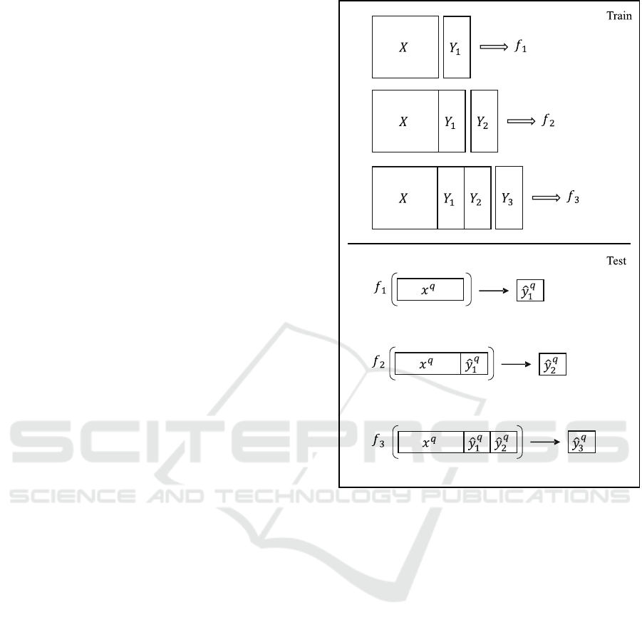
Graphical illustration of RC is shown in Figure 2.
In the illustration, there are three output (target) vari-
ables (y
1
, y
2
, and y
3
) and training input data (X). In
the first stage of training process starts with fitting a
model (f
1
) for the first output variable (y
1
) by using
base inputs (X). Then, in the second stage, a new
model (f
2
) is fitted for the second output variable (y
2
)
by using modified input that is created with concate-
nating base inputs (X) and the actual values of the first
output (y
1
). Finally, f
3
is created by using the third
output variable (y
3
) and concatenated data (X,y
1
, and
y
2
) in the third stage.
In testing process, predictions for the first output
(ˆy
q
1
) are made by using (f
1
). Then, the first predic-
tions are added to the test input data (x
q
), and it is
used for predicting the second output (ˆy
q
2
) by model
(f
2
). In the last step, first two predictions (ˆy
q
1
, and ˆy
q
2
)
concatenated with the test input data (x
q
), and ˆy
q
3
is
predicted by model 3 (f
3
).
The main problem of this method is that the ran-
domness in determining chain sequence causes signif-
icant differences in predictive performance. In order
to avoid this problem, ERC method is proposed by
(Spyromitros-Xioufis et al., 2012). The ERC method
suggests using a set of regression chains consisting of
all possible chains or a group of chains which is ran-
domly selected if the output dimension is too high,
in an ensembled structure. After determining the set
of chain sequences, the ERC approach predicts the
target variable for each stage of the chain and finally
presents their averages as predicted values for each
target variable.
The difference between RC and ERC is that RC
takes the single prediction for each output in a certain
sequence. However, ERC makes predictions for all
permutations of sequence and gives the final predic-
tion as the average of all predictions for each output.
2.3 Predictive Models
MTR is a meta-learner which can use different es-
timators and set of learning sequences in a pre-
determined configuration. In this part, we introduce
three common regression techniques to conduct a
benchmark test and determine the most appropriate
one to apply our dataset. These estimators are: 1) De-
Figure 2: Graphical illustration of RC.
cision Tree Regressor, 2) Random Forest Regressor,
and 3) Multivariate Adaptive Regression Splines.
2.3.1 Decision Tree Regressor
Decision Tree induction is one of the most important
supervised learning methods which is used for clas-
sification and regression. Decision Tree Regressor
constructs a flowchart-like structure where each in-
ternal (non-leaf) node denotes a test on an attribute,
each branch corresponds to an outcome of the test,
and each external (leaf) node denotes a class predic-
tion. At each node, the algorithm chooses the “best”
attribute to partition the data into individual classes
(Han et al., 2011). The main idea here is to create
a decision tree model that minimizes error on each
leaf. Different algorithms may be applied to build
decision threes such as Classification and Regression
Trees (CART) which uses Gini Index as metric and
Iterative Dichotomiser 3 (ID3) which uses Entropy
function and Information gain as metrics (Quinlan,
1986). We used Gini method in CART algorithm.
Ensemble Learning based on Regressor Chains: A Case on Quality Prediction
269
2.3.2 Random Forest Regressor
Random Forest is an ensemble learning method that
aims to improve predictiveaccuracy and preventover-
fitting by fitting multiple decision trees on various
sub-samples of the dataset and combining them un-
der a single meta-estimator (Breiman, 2001). Ran-
dom Forest Regressor (RF) uses the average predic-
tion for regression of trees which are constructed by
training on different data sample. These samples are
created by Bootstrap Aggregation (or bagging).
2.3.3 Multivariate Adaptive Regression Splines
Multivariate Adaptive Regression Splines (MARS)
is a non-parametric extension of the standard linear
model without any assumption about the underlying
functional relationship between the dependent and in-
dependent variables. MARS model is obtained by
using combination of piece-wise basis functions, for-
ward and backward passing procedures in the regres-
sion models. Each term in a MARS model is a prod-
uct of so called “hinge functions”. A hinge function
is a function that’s equal to its argument where that
argument is greater than zero and is zero everywhere
else (Friedman et al., 1991).
MARS builds a model which is formed follow-
ingly:
f(x) =
k
∑
i=0
c
i
B
i
(x
i
), (1)
where x is a vector of sample features, B
i
is a piece-
wise function that consists of a set of basis functions
and c
i
the coefficient. Basis function may behave in
three different ways based on the input range: First, it
can be constant 1, to reduce bias. Second, it can be a
hinge function h(x) = max(0, x −t) or max(0,t −x),
where t is a constant, so the model represents non-
linearities. Third, it can be a product of multiple hinge
functions to combine interactions between features.
3 EXPERIMENTAL SETUP
3.1 Dataset
In this study, we apply the algorithms to dataset ob-
tained from paired process data (signals) of textile
manufacturing. There are total of 1,511 rows, one row
for each lab sample in dataset, and each lab sample
has 19 signal values, such that weaving speed, tem-
perature, and yarn tension, as input for algorithms;
and 3 quality metrics, water permeability (Metric 1),
tear strength (Metric 2), and abrasion resistance (Met-
ric 3), that are obtained after lab sample assessed in
the laboratory as output of algorithms.
The statistical summary of the 19 features is
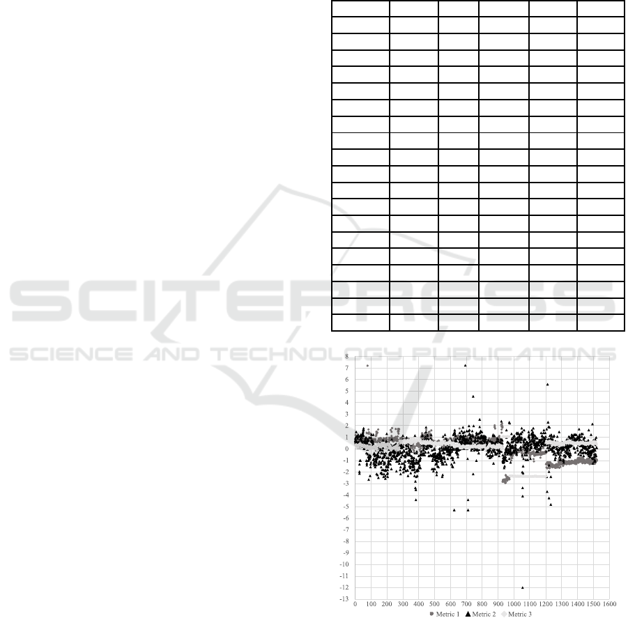
shown in Table 1. Also, the Z-normalization of tar-
get metrics 1, 2 and 3 is given in Figure 3.
Table 1: Feature Summary Statistics.
Feature Mean Std CoV* Min Max
0 70.0 1.0 0.0 65.7 74.5
1 -10.8 1.2 -0.1 -14.5 -7.7
2 -4.2 1.2 -0.3 -8.5 -2.2
3 -0.2 0.1 -0.3 -0.4 0.0
4 -0.3 0.2 -0.5 -0.3 0.0
5 7.4 2.1 0.3 0.0 14.8
6 31.9 2.6 0.1 28.5 53.7
7 302.9 77.1 0.3 198.9 401.4
8 27.2 0.0 0.0 27.2 27.2
9 37.9 0.0 0.0 37.9 37.9
10 25.2 2.8 0.1 20.3 31.8
11 49.9 4.1 0.1 42.3 57.3
12 63.0 6.9 0.1 44.4 70.4
13 28.3 1.6 0.1 23.2 32.3
14 25.3 2.2 0.1 18.8 31.8
15 152.6 4.9 0.0 143.4 163.7
16 146.5 8.8 0.1 119.1 154.6
17 225.8 0.6 0.0 225.1 226.3
18 20.7 1.5 0.1 17.7 25.2
*CoV: Coefficient of Variation
Figure 3: Distribution of Target Data.
After examining the target data, it is observed that
the variance of Z-values of Metric 2 is much higher
than that of other metrics. Feature importance anal-
ysis is performed for each metric to see whether the
characteristics of Metric 3 shows similarities in terms
of ability to be expressed by features. Analysis results
DATA 2019 - 8th International Conference on Data Science, Technology and Applications
270
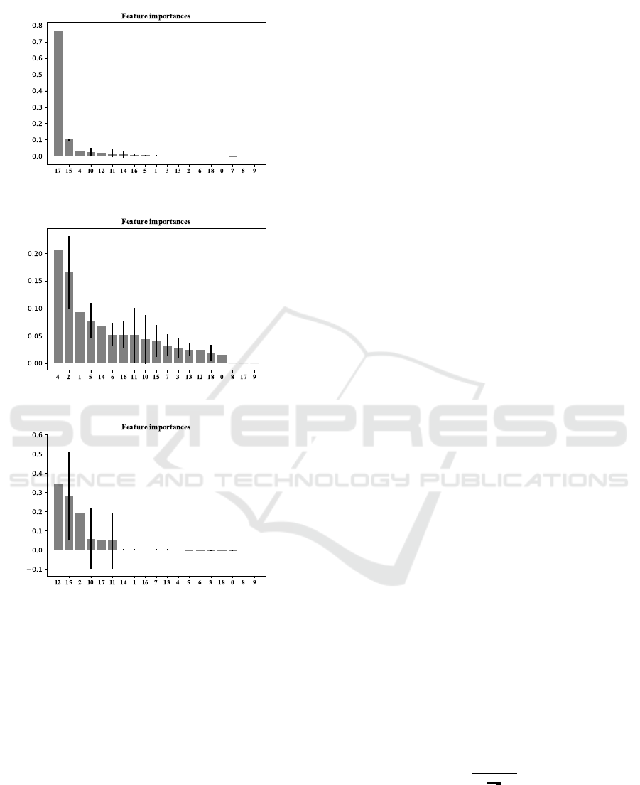
can be seen in Figure 4, 5 and 6.
Figure 4: Feature Importance of Metric 1.
Figure 5: Feature Importance of Metric 2.
Figure 6: Feature Importance of Metric 3.
According to the feature importance analysis,
while there are at least one features have minimum
of 20% importance on Metric 1 and 3, the importance
rate of all features are less than 20% for Metric 2. In
this sense, it can be concluded that Metric 2 is dis-
advantageous compared to other metrics in terms of
both the distribution character and the power to be ex-
pressed by existing feature set.
3.2 Outlier Detection
In order to obtain the most suitable models for the
natural characteristics of production process, the data
is divided into clusters according to the Local Outlier
Factor (LOF) method (Breunig et al., 2000). For any
given data instance, the LOF score is equal to ratio of
average local density of the k-nearest neighbors of the
instance and the local density of the data instance it-
self (Chandola et al., 2009). The local density of each
sample is compared with the local densities of the
neighbors and the samples with significantly lower
density than their neighbors are specified as outliers.
In this study, the number of neighbors, k, is assumed
as 10, and the cluster which has greatest dissimilar-
ity is extracted and labeled as “unusual”. Segmen-
tation yields two segments of size 1,431 (“normal”
segment) and 80 (“unusual” segment). We divide the
“normal” dataset further into training and testing sets,
which have 1,144 and 287 data points respectively.
In the next section, we use several machine learn-
ing algorithms and compare their prediction perfor-
mance using a series of statistical analysis. The anal-
ysis conducted in two major steps. First, analysis
regarding the “normal” data is presented. Then, the
analysis for the “unusual” data is presented, where it
is seen that the ensemble of regressor chains signifi-
cantly outperforms the single target model.
3.3 Implementation and Analysis
In the first step of the numerical analysis, single-target
regression models are created for each metric in the
“normal” dataset. Then, the best performing single-
target regression model is selected to be compared
with the ERC model. During the comparisons, we use
MAPE as the key performance metric and conduct a
set of statistical tests/analysis, which are vector com-
parison, paired t-test and one-way ANOVA test. In
the second step, similar comparison between single-
target regression model and ERC is conducted using
the “unusual” dataset.
For the sake of completeness, we present the de-
tails of the metrics, statistical tests and analysis we
use during the comparison.
In paired t-test, the mean of the observed values
for a variable from two dependent samples are paired
and compared. As we use different algorithms to pre-
dict the same set of data points, pairing is direct pos-
sible as a natural consequence of the process. The test
is used to decide whether the sample means compared
are identical or not. The differences between all pairs
are calculated by the following equation:
t =
¯
X
D
−µ
0
s
D
√
n
., (2)
where
¯
X
D
and s
D
are the mean and standard devia-
tion of those differences, respectively. The constant
µ
0
equals to zero if the underlying hypothesis assumes
the two samples are coming from populations with
identical means, and n represents the number of pairs.
Ensemble Learning based on Regressor Chains: A Case on Quality Prediction
271
The one-way ANOVA test compares whether
mean of two or more samples are the same. The main
assumptions of ANOVA test is that the distribution of
each sample is normal and the samples are indepen-
dent.
In vector comparison analysis, algorithms are
scored for their prediction performance for each and
every data point separately. The algorithm yielding
the minimum absolute percentage error for the given
data point receives 1 (winner), others receive 0. Test
results for MAPE comparison, vector comparison and
t-test comparison are given in Table 2, Table 3, Table
4 and Table 5 respectively. In Table 2, test and (train)
errors are given respectively.
Table 2: MAPE Comparison for ST Models.
RF DTR MARS
Metric 1 0.020 0.023 0.027
(0.011) (0.017) (0.024)
Metric 2 0.045 0.046 0.047
(0.030) (0.044) (0.046)
Metric 3 0.003 0.030 0.007
(0.002) (0.030) (0.007)
Table 3: Vector Comparison.
RF DTR MARS
Metric 1 126 78 83
Metric 2 95 104 88
Metric 3 132 107 48
Table 4: Paired t-test Comparison.
y− ˆy
RF
y− ˆy
DTR
y− ˆy
MARS
Metric 1 0.818 0.694 0.914
Metric 2 0.621 0.459 0.536
Metric 3 0.982 0.398 0.275
Table 5: One-way ANOVA Comparison.
p-value
Metric 1 0.935
Metric 2 0.983
Metric 3 0.308
When the MAPE values are examined, it is ob-
served that the values are very close to each other
but the best test results are obtained by RF for three
metrics. The best results for Metric 1 and Metric 3
are taken by RF in the vector comparison, whereas
MARS model predicted nine lab samples better than
RF for Metric 2.
Paired t-test results presented in Table 4 reveal
that all predictions yielded residuals with zero mean.
For the constant variation assumption, RF model’s
residual vs. fitted plot for Metric 2 is presented in
Figure 7. Figure 7 reveals that there is no indication
for the violation of constant variation assumption.
Following these, analyzes it is determined that
working with RF would be more appropriate for this
dataset and it is chosen as the baseline model.
The noteworthy point here is that the MAPE value
of Metric 2 is higher than MAPE values of other two
variables. In order to better understand the relation-
ship between outputs, correlation between the output
values are measured and it is seen that there is no lin-
ear relationship between the output of Metrics 1-2 and
2-3 as shown in Table 6.
Table 6: Correlation Matrix of Output Variables.
Metric 1 Metric 2 Metric 3
Metric 1 1 -0.019 0.018
Metric 2 -0.019 1 -0.200
Metric 3 0.018 -0.200 1
At this point, multi-output regression approach
can be seen as an opportunity to improve the rela-
tively bad performance we observe for Metric 2. With
the regressor chains method, all input and output vari-
ables can be evaluated together, thus the dependencies
and internal relationships between them that have a
positive impact on the predictive performance may be
unveiled (Borchani et al., 2015). Since we have small
number of outputs, regression models are trained for
all possible chain sequences by applying the ERC
framework, and the mean of the predicted values from
each model are recorded as final predictions. MAPE
comparison, vector comparison and paired t-test re-
sults are shown in Table 7, Table 8 and Table 9.
Table 7: ERC vs ST Mape Comparison for testing.
ERC ST
Metric 1 0.019 0.020
Metric 2 0.042 0.045
Metric 3 0.003 0.003
Table 8: ERC vs ST Vector Comparison for testing.
ERC ST
Metric 1 159 129
Metric 2 150 138
Metric 3 133 155
According to Table 7, ERC approach provides %5
and %4.5 improvement over the performance of ST
in predicting Metric 1 and Metric 2 respectively. The
benefit of the ERC approach for Metric 1 and 2 is also
obvious in the vector comparison test. For Metric 3,
on the other hand, the number of predictions with im-
proved error value is small. This can be explained by
the fact that the given MAPE value is already very
low for that metric. In other words, we can conclude
DATA 2019 - 8th International Conference on Data Science, Technology and Applications
272
that Metric 3 is easy to predict compared to predicting
Metric 1, and especially Metric 2. It is seen in Table 9
that there is no evidence to conclude that ERC method
is superior to ST method in predicting Metric 1 and
3, since the p-values for the test statistic for compar-
ing residual vectors for ERC and ST are larger than
the conventional significance level threshold 0.05. On
the other hand, result for Metric 2 conveys a different
message. It is seen that prediction performance ERC
is signficantly better that of ST at 0.05 significance
level.
Table 9: ERC vs ST residuals t-test Comparison for testing.
~
R
i
j
represents residual vector of algorithm i for metric j.
Residuals p-Value
~
R
ERC
1
−
~
R
ST
1
0.115
~
R
ERC
2
−
~
R
ST
2
0.025
~
R
ERC
3
−
~
R
ST
3
0.382
In the second phase of the analysis, the effect of
the ERC approach on predictive performance is mea-
sured for “unusual” dataset. Since this piece of the
dataset is outside of the general production character-
istics, it is obvious that the regression models which
are trained by the data that has usual production pa-
rameters will give worse results for this set.
The results of Metric 2, which are already rela-
tively poor, will be worsened for the “unusual” data
segment. However, with ERC approach, the unveiled
internal relations between target and input variables
provide some improvement in the prediction accu-
racy. Comparison results are presented in Table 10,
Table 11 and Table 12.
It is seen in MAPE comparison table that ERC ap-
proach provides %6.9, %8 improvement for Metric 1
and 2, respectively. The apparent superiority of the
ERC approach compared to the ST is clearly seen in
vector comparisons as well. For Metric 2, ST beats
ERC in prediction of only 29 samples, whereas the
ERC beats ST in 51 samples. It is seen in Table 12
if the significance level is chosen tobe 0.1, then ERC
dominates ST in all three metrics. On the other hand,
when the significance level is set to 0.05, then we may
say there is not enough evidence to conclude that ERC
method is superior to ST method in predicting Metric
3. However, for Metric 1 and 2, ERC significantly
outperfoms in ST approach even at 0.05 threshold.
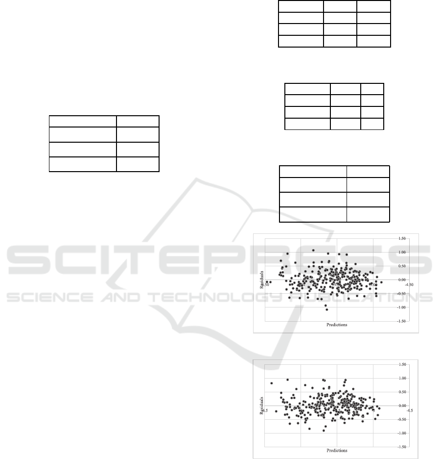
As the final analysis, we present residual vs. fitted
plots for i) ST and ERC models (for Metric 2 under
“normal” test dataset) in Figure 7 and Figure 8; and
ii) ST and ERC models (for Metric 2 under “unusual”
test dataset) in Figure 9 and Figure 10 . Residual anal-
yses of ST and ERC for other metrics (for both normal
and unusual test datasets) are behaving similar char-
acteristics.
Table 10: ERC vs ST Mape Comparison for unusual seg-
ment.
ERC ST
Metric 1 0.027 0.029
Metric 2 0.127 0.138
Metric 3 0.004 0.004
Table 11: ERC vs ST Vector Comparison for unusual seg-
ment.
ERC ST
Metric 1 43 37
Metric 2 51 29
Metric 3 44 36
Table 12: ERC vs ST residuals t-test Comparison for un-
usual segment.
Residuals p-Value
~
R
ERC
1
−
~
R
ST
1
0.006
~
R
ERC
2
−
~
R
ST
2
0
~
R
ERC
3
−
~
R
ST
3
0.078
Figure 7: ST-Prediction vs Residuals for Metric 2 in testing.
Figure 8: ERC-Prediction vs Residuals for Metric 2 in test-
ing.
It is seen in Figure 7 and Figure 10 that resid-
uals are scattered randomly around mean zero with
constant variance. This indicates that both predictive
models are adequate in modeling the variation in the
response variables in “normal” test data.
Similar to the above discussion, it is seen Figure 7
and Figure 10 that residuals can be assumed to have
Ensemble Learning based on Regressor Chains: A Case on Quality Prediction
273
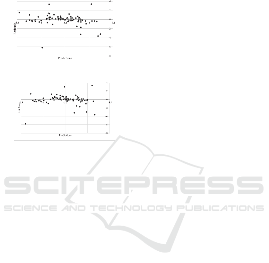
Figure 9: ST-Predictionvs Residuals for Metric 2 in unusual
segment.
Figure 10: ERC-Prediction vs Residuals for Metric 2 in un-
usual segment.
zero mean value and show a constant variation be-
haviour, which is again can be seen as an indication
that both predictive models are adequate in modeling
the variation in the response variables in ”unusual”
test data. Although we observe some outliers in the
residuals. we could say that this is normal consider-
ing that the ”unusual” dataset is statistically different
than the dataset we train our machine learning algo-
rithms.
4 CONCLUSION
In this paper we proposedan ensemble machine learn-
ing algorithm in order to predict the finished yarn
quality. The data is first segmented into ten clusters
nine of which is denoted as ”normal” and the one
with the highest distance from the general mean as
”unusual” via local outlier factor method. The former
cluster refers to production data one may expect due
to the nature of the process and latter is the dataset
showing an usual pattern compared to expected pro-
cess data. Then a set of classical machine learning
algorithms are applied and performances of the algo-
rithms is compared. It is seen that for the unusual
segment, performance of the classical algorithms gets
worse especially for one of the quality metrics. As
a remedy, an ensemble algorithm based on regressor
chains is recommended and yielding higher predic-
tion performance in two thirds of the dataset.
As the next step, implemented algorithm will be
fully tested at the facility. If the prediction perfor-
mance remains satisfactory, we’re going to move on
the next phase and start using the predictive tool as a
recommendation engine for the machine operator. At
this stage, operator will be informed about the sug-
gested production settings for the machine and the
recommendation system will perform as a decision
support tool, meaning that the recommendations of
the tool are push forward to the machine only if the
operator gives consent. Once the second phase is suc-
cessful, the recommendation engine will be plugged
into PLC and start changing set parameters of the ma-
chine as a part of the automation system. After the
third phase, the manufacturing plant will have its first
full-scale industry 4.0 application.
REFERENCES
Borchani, H., Varando, G., Bielza, C., and Larra˜naga, P.
(2015). A survey on multi-output regression. Wiley
Interdisciplinary Reviews: Data Mining and Knowl-
edge Discovery, 5(5):216–233.
Breiman, L. (2001). Random forests. Machine learning,
45(1):5–32.
Breunig, M. M., Kriegel, H.-P., Ng, R. T., and Sander, J.
(2000). Lof: identifying density-based local outliers.
In ACM sigmod record, volume 29, pages 93–104.
ACM.
Chandola, V., Banerjee, A., and Kumar, V. (2009).
Anomaly detection: A survey. ACM computing sur-
veys (CSUR), 41(3):15.
De’Ath, G. (2002). Multivariate regression trees: a new
technique for modeling species–environment relation-
ships. Ecology, 83(4):1105–1117.
Friedman, J. H. et al. (1991). Multivariate adaptive regres-
sion splines. The annals of statistics, 19(1):1–67.
Han, J., Pei, J., and Kamber, M. (2011). Data mining: con-
cepts and techniques. Elsevier.
Quinlan, J. R. (1986). Induction of decision trees. Machine
learning, 1(1):81–106.
Simil¨a, T. and Tikka, J. (2007). Input selection and shrink-
age in multiresponse linear regression. Computational
Statistics & Data Analysis, 52(1):406–422.
Spyromitros-Xioufis, E., Tsoumakas, G., Groves, W.,
and Vlahavas, I. (2012). Multi-label classification
methods for multi-target regression. arXiv preprint
arXiv:1211.6581, pages 1159–1168.
Struyf, J. and Dˇzeroski, S. (2005). Constraint based induc-
tion of multi-objective regression trees. In Interna-
tional Workshop on Knowledge Discovery in Inductive
Databases, pages 222–233. Springer.
Vazquez, E. and Walter, E. (2003). Multi-output supp-
port vector regression. IFAC Proceedings Volumes,
36(16):1783–1788.
Zhang, W., Liu, X., Ding, Y., and Shi, D. (2012). Multi-
output ls-svr machine in extended feature space.
In 2012 IEEE International Conference on Compu-
tational Intelligence for Measurement Systems and
Applications (CIMSA) Proceedings, pages 130–134.
IEEE.
DATA 2019 - 8th International Conference on Data Science, Technology and Applications
274
