Hybrid 6D Object Pose Estimation from the RGB Image

Rafal Staszak

and Dominik Belter

Institute of Control, Robotics and Information Engineering, Poznan University of Technology, Poznan, Poland

Keywords:

Object Pose Estimation, Convolutional Neural Networks, Deep Learning in Robotics.

Abstract:

In this research, we focus on the 6D pose estimation of known objects from the RGB image. In contrast to

state of the art methods, which are based on the end-to-end neural network training, we proposed a hybrid

approach. We use separate deep neural networks to: detect the object on the image, estimate the center of the

object, and estimate the translation and ”in-place” rotation of the object. Then, we use geometrical relations on

the image and the camera model to recover the full 6D object pose. As a result, we avoid the direct estimation

of the object orientation deﬁned in SO3 using a neural network. We propose the 4D-NET neural network to

estimate translation and ”in-place” rotation of the object. Finally, we show results on the images generated

from the Pascal VOC and ShapeNet datasets.

1 INTRODUCTION

Collaborative robotic arms are designed to share

workspace with humans or even physically interact

with operators. This is possible mainly due to con-

trol algorithms which make the robot compliant when

robot unexpectedly touches an obstacle. Also, simple

safety sensors stop or slow down the robot when the

human operator get too close to the dangerous area.

These types of robot become very popular in man-

ufacturing to perform repetitive tasks. In our research,

we are interested in the autonomy of such robots. A

collaborative arm, which is mounted on the mobile

platform, can move freely in the factory and perform

production tasks or help humans in daily activity. To

this end, the mobile robot should be equipped with

the perception system which allows detecting and es-

timating the pose of the objects and then perform ma-

nipulation tasks (Fig. 1).

In this paper, we consider the problem of visual

objects detection and pose estimation. Most of the

state of the art methods are based on the visual or

depth features (Hinterstoisser et al., 2012; Hodan

et al., 2015), which are used to detect and ﬁnd the

6D pose (position and orientation) of the object. Re-

cently, great progress was made in this ﬁeld. Kehl et

al. (Kehl et al., 2017) showed that the Deep Convolu-

tional Neural Network can be applied to detect objects

on the RGB images and simultaneously estimate the

https://orcid.org/0000-0002-5235-4201

https://orcid.org/0000-0003-3002-9747

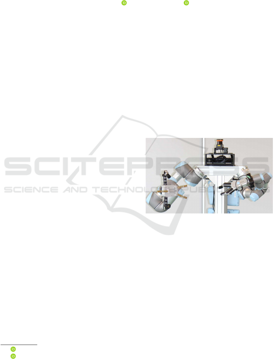
Figure 1: Mobile-manipulating robot used in this research

equipped with RGB-D cameras mounted in robot’s head

and wrists.

pose of the object. On the other hand, the traditional

methods based on online optimization have proven

to be very efﬁcient. (Bibby and Reid, 2016; Tjaden

et al., 2016; Prisacariu and Reid, 2012). Bibby et al.

propose the object tracking method which minimizes

the error deﬁned directly on the RGB image. The

silhouette generated from the object model is com-

pared with the intensity of pixels on the current im-

age. The pose of the object model is modiﬁed using

the gradient-based method. The algorithm is designed

for object tracking. It means that the algorithm re-

quires a very accurate initial guess and can’t be used

for object detection.

In this research, we propose a new hybrid method

for 6D object pose estimation (3D translation and ro-

tation). In contrast to end-to-end solutions, we pro-

pose a method which utilizes deep neural network

Staszak, R. and Belter, D.

Hybrid 6D Object Pose Estimation from the RGB Image.

DOI: 10.5220/0007933105410549

In Proceedings of the 16th International Conference on Informatics in Control, Automation and Robotics (ICINCO 2019), pages 541-549

ISBN: 978-989-758-380-3

541

pose estimator and a geometrical model of the cam-

era.

1.1 Related Work

Many traditional approaches to 6D objects pose es-

timation are based on visual RGB or depth features.

Then, the features are compared with the reference

models to produce an object category and pose esti-

mation. In (Hinterstoisser et al., 2012), which is an

extension of the LINEMOD method (Hinterstoisser

et al., 2011), the color gradient features located on

the object silhouette and surface normal features in-

side the object silhouette are selected to describe dis-

cretized object pose. The detector is trained using

texture-less 3D CAD models of the objects. In (Ulrich

et al., 2012) RGB edges are used for objects detection

and pose estimation. The pose estimation is boosted

by the hierarchical view model of the object (Ulrich

et al., 2012). Hodan et al. propose a sliding window

detector based on surface normals, image gradients,

depth, and color (Hodan et al., 2015). The pose of

the object is estimated using a black-box optimization

technique (Particle Swarm Optimization) which mini-

mizes the objective function deﬁned using the current

depth image and the synthetic image generated from

the CAD model of the object.

To detect an object in the image a Random For-

est classiﬁer can be used (Brachmann et al., 2016).

The obtained distribution of object classes is used to

obtain preliminary pose estimates for the object in-

stances. Then, the initial poses are reﬁned using ob-

ject coordinate distributions projected on the RGB

image. Similar Latent-Class Hough Forests allow

learning the pose estimator using RGB-D LINEMOD

features (Tejani et al., 2016).

Another method for pose estimation is Iterative

Closest Point algorithm (Segal et al., 2009). In con-

trast to previously mentioned methods, the ICP relies

on depth data (point clouds). In practice the point

cloud obtained from popular Kinect-like sensors are

noisy. We avoid using depth data and rely mainly on

the RGB images for pose estimation because the er-

ror of the single depth measurement can be larger than

5 cm on our depth sensor (Kinect v2) (Khoshelham,

2011). We also avoid methods similar to ICP because

they are very sensitive to initial guess about the object

pose. The initial pose of the object should be close to

the real pose of the object because the ICP is prone to

local minima.

Another group of object detection methods is

based on Deep Convolutional Neural Networks. Kehl

et al. (Kehl et al., 2017) proposed the extension to

the Single Shot Detector (SSD) (Liu et al., 2016), to

detect the position of the objects on the image and

produces 6D pose hypotheses of the objects. The net-

work is trained using synthetic images generated from

the MS COCO dataset images as a background and

3D CAD models of the objects. The 6D pose hy-

potheses of each object are later reﬁned using RGB-D

images.

Also, Xiang et al. use a Convolutional Neural Net-

work to estimate the 6D pose of the objects from the

RGB image (Xiang et al., 2018). In this case, the es-

timation of translation and rotation of the object is

decoupled. To estimate the translation of the object

the neural network estimates the center of the object.

Then, the translation of the object is computed from

the camera model. The orientation of the object is es-

timated by the neural network working on the Region

of Interests (bounding boxes) detected on the input

image. In the method proposed by Thanh-Toan Do et

al., the neural network estimates the distance to the

camera only (Do et al., 2018). The remaining compo-

nents of the translation vector are estimated from the

bounding box. The rotation of the object is estimated

using Lie algebra representation.

Estimation of the orientation of the object is the

most challenging part of the 6D pose estimation.

In (Sundermeyer et al., 2018) the orientation of the

object is deﬁned implicitly by samples in latent space.

Utilizing the depth data improves the results (Wang

et al., 2019) but also template matching-based method

has been proven to be efﬁcient in this case (Konishi

et al., 2018).

To deal with the 6D pose estimation we decouple

the solution into two sub-problems. First, we use the

neural network to ﬁnd the pose of the object with re-

spect to the camera frame assuming that the camera

axis goes through the center of the object. Then, we

analytically correct the estimated pose of the object

using camera model. Moreover, we have used degen-

erated representations for describing 6D pose in order

to simplify speciﬁc tasks.

2 4D-2D POSE ESTIMATION

Given an RGB input image, the task of pose estima-

tion pipeline is to estimate the rigid transform be-

tween coordinate systems O and C belonging to the

object and the camera, respectively. We state that

the full representation of the rigid transform can be

retrieved through an ensemble of speciﬁc tasks with

reduced dimensionality. The ﬁrst constraint reduc-

ing the dimensionality to four parameters is the re-

lation between the z-axis of C coordinate system and

the origin position of O coordinate system. If we as-

ICINCO 2019 - 16th International Conference on Informatics in Control, Automation and Robotics

542

sume that the z-axis belonging to C intersects the ori-

gin of O coordinate system then it is possible to cre-

ate a rigid transform using only four parameters: XYZ

translation and in-place rotation angle θ. The XYZ

translation determines the location of camera as well

as the direction of its z-axis. The x and y axes of the

camera rigid transform depend on the in-place rota-

tion angle. It can be perceived as a tilt movement of

camera. in-place rotation angle determines the mea-

sure of camera rotation around its z-axis.

The neural network estimates transformation be-

tween the camera C

and the object frame O. Because

we assume that the z axis of the C

frame goes through

the center of the object frame O the neural network

has to estimate only four parameters. The natural

choice is the representation with three Euler angles

and distance to the object z. In this case, x and y is al-

ways zero. However, the Euler angles are not the best

choice to represent the orientation of the object be-

cause of singularities and nonlinearity. Another possi-

bility is to represent the pose of the object by the axis-

angle representation and distance to the object. How-

ever, we chose the representation which contains three

parameters deﬁned in the Euclidean space (translation

from the object frame O to the camera frame C

) and

the in-place rotation angle θ. As it was stated before

the translation represents the position of the camera

on a spherical surface around the object and the θ an-

gle represents the rotation around z axis of the camera.

The rotation angles around x and y axis of the camera

frame C

are always set to zero because the camera

axis z goes through the center of the object. Finally,

our neural network estimates three parameters deﬁned

in the Euclidean space avoiding the ambiguities of the

Euler angles representation.

The imposed constraint assumes that the object is

always located in the image center. Therefore we can

obtain the two lost degrees of freedom by determining

the object center expressed in image coordinates and

reﬁne the pose. Thus, the resultant coordinate system

C’ deﬁned by XYZR vector can be reﬁned by rotating

it to make its z-axis intersect the image center.

2.1 Methodology

Let C denote a rigid transform between the object

and the camera coordinate system given by O and C,

which are shown in Fig. 2 Apart from that let C

de-

note a rigid transform whose z-axis intersects the ori-

gin of the O coordinate system. The homogeneous

matrix representation of C

is derived from transla-

tion vector C

and in-place rotation angle θ. In order

to determine the matrix representation of C

we as-

sume that the x-axis of camera coordinate system is

parallel to the O

plane if θ equals zero. Given these

assumptions we determine C

as follows:

z =

||C

, (1)

x =

[−z

,0]

+ z

, (2)

y = z × x, (3)



x y z C

0 0 0 1









.cos(θ) −sin(θ) 0 0

sin(θ) cos(θ) 0 0

0 0 1 0

0 0 0 1







(4)

The method of calculating the x vector leads to a sin-

gularity when the ﬁrst two components of z vector

equal zero. In practical implementation it is very un-

likely for a neural network to output such values of its

rarity in single-precision ﬂoating-point number for-

mat. However, we assign a constant value to x in order

to ensure that the computation will not fail.

Further calculation of the goal representation of C

rigid transform can be carried out when the relevant

camera parameters are known. Let w,h be the width

and height of images produced by the camera. Addi-

tionally the camera parameters are deﬁned by f

and

which denote camera ﬁeld of view for width and

height, respectively. If we know the actual position

of the object’s centre on the image I, then the cor-

rection T that should be applied is represented by:



−



· f



−



· f

T =







cos(φ

) 0 sin(φ

) 0

0 1 0 0

−sin(φ

) 0 cos(φ

) 0

0 0 0 1













1 0 0 0

0 cos(φ

) −sin(φ

) 0

0 sin(φ

) cos(φ

) 0

0 0 0 1







(5)

2.2 Architecture

The whole pipeline for 6D pose estimation presented

in Fig. 3 consists of three modules: object extrac-

tor (Mask R-CNN (He et al., 2017)), camera coarse

Hybrid 6D Object Pose Estimation from the RGB Image

543

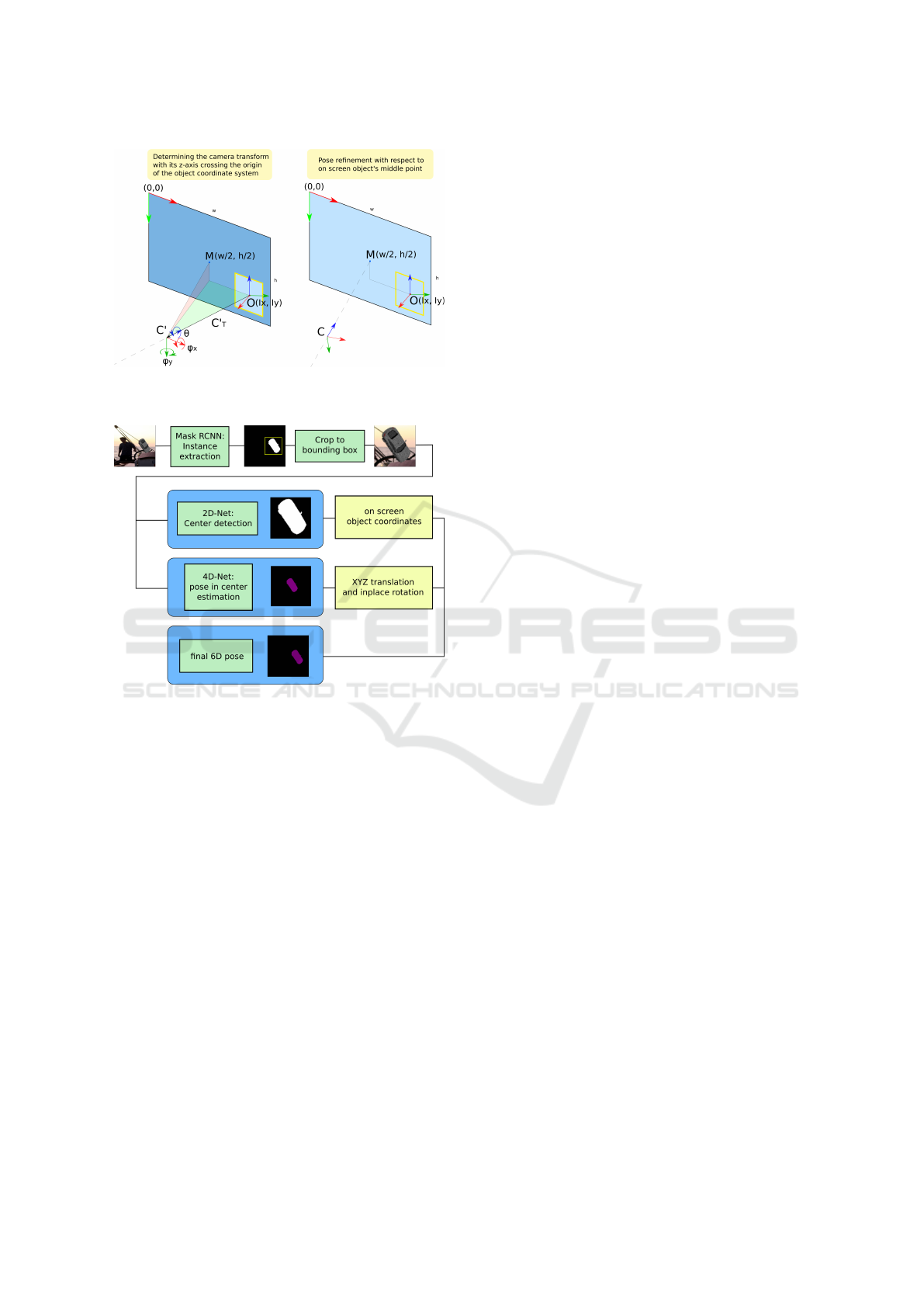
Figure 2: Visualization of the consecutive steps of our pose

estimation approach.

Figure 3: The pipeline of the 6D pose estimation frame-

work.

position estimator (4D-NET) and object’s centre es-

timator (2D-NET). In practice, the object can be lo-

cated in any random position on an image plane. With

no prior knowledge as to where the object is located

and what area it covers it is complicated to predict

the pose precisely. Object extraction is therefore of

paramount importance, since the ratio of relevant and

irrelevant information might be very low given the

full, uncropped image. Furthermore, the image may

contain several objects and every one of them should

be addressed separately.

The image extractor’s main task is to provide de-

tailed image and class information about objects in

the scene. The modules responsible for parameter es-

timation are trained separately for every single object.

The class information derived from the image extrac-

tor serves as a selector for the modules that should be

run to analyze the image excerpt.

2.3 Object Extractor

The ﬁrst network in the pipeline is the object extrac-

tor. The object extractor is fed by RGB data and out-

puts the mask and bounding box information about all

the detected objects. We use the Mask R-CNN archi-

tecture which provides the 2D mask, class informa-

tion and bounding boxes of objects (He et al., 2017).

After successful detection all the objects are cut out

from the image according to their bounding boxes.

The input shape of 4D-NET and 2D-NET is constant

and square which involves reshaping bounding boxes

in order to match the dimensions.

2.4 4D-NET Architecture

The architecture of the 4D-NET is presented in Fig.

4. The base of the network is built in a fully convolu-

tional manner. The input of the network has a shape of

64 × 64 × 3. We use strides of 1 and kernel of shape

3 × 3 across the whole network. We apply weights

regularization according to the L2 rule with a scale

coefﬁcient set to 0.01. At the beginning of the train-

ing weights are initialized with the usage of Xavier

initializer. The reasons behind a convolutional-based

architecture are its proven capabilities of separating

relevant image data and overall generalization prop-

erties. The output of the last convolutional layer is

ﬂattened and fed then to another two fully connected

layers with 512 and 4 units. The latter layer provides

a prediction of relative translation from the camera to

the object as

T coordinates and in-place rotation an-

gle θ. In order to avoid overﬁtting the convolutional

layers are trained with batch normalization technique

and the fully connected layers apply dropout omitting

half of the connections. The ReLU activation function

is used across the entire network.

2.5 4D-NET Loss Function

Since the goal of estimating XYZ translation and in-

place rotation angle is to determine the C

rigid trans-

form we have decided not to treat each parameter sep-

arately but rather couple them all together. Impre-

cise XYZ prediction results in an increasing angle

error between target and predicted rigid transforms

when we compare them in angle-axis representation.

With that in mind, we have introduced a loss func-

tion which penalizes the network for any trial to com-

pensate the distance error at the expense of rotation.

Moreover, the order of magnitude of translation error

may vary signiﬁcantly within the dataset. This kind

of data instability is alleviated by varying normalizing

ICINCO 2019 - 16th International Conference on Informatics in Control, Automation and Robotics

544

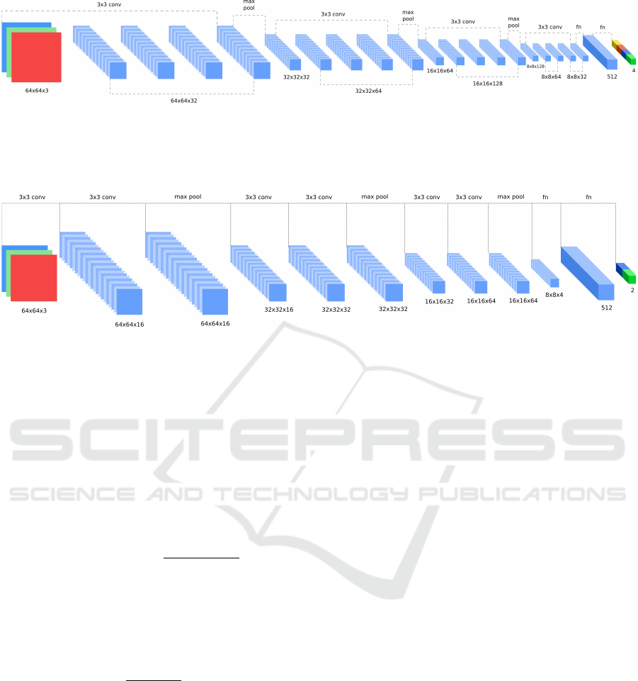
Figure 4: The architecture of 4D-NET. The network takes as input a three-channel color image and converts it into four-

element vector through consecutive convolutional and two dense layers. The resultant vector consist of relative camera to

object XYZ translation and in-place rotation angle.

Figure 5: The architecture of 2D-NET. The input of 2D-NET is a three-channel color image, same as in 4D-NET, and it

outputs a two-element vector, which describes the center of the object projected on the image plane. The image coordinates

are normalized during training and the network outputs values within a range of 0 to 1.

term which is directly dependent on the translation la-

bel.

Let T,

T,R,

R denote the target and predicted

translation vectors and the rigid transforms’ rotation

matrices. The function G(R,

R) deﬁnes the angle dif-

ference between target and predicted rotation matrices

in angle-axis representation:





= arccos



R ·



− 1

. (6)

The overall loss function is a sum of resultant dis-

tance and rotation errors. The λ coefﬁcient has been

added in order to weigh the practically incomparable

distance and rotation measures:

`(T,

T , R,

R) =

||T −

T ||

||T ||

+ λ · G





. (7)

2.6 2D-NET Architecture

The architecture of the 4D-NET is presented in Fig. 5.

The architecture of the network consists of 6 con-

volutional, 3 pooling and 2 fully connected layers.

The network uses strides of 1 and kernels of shape

3x3 for convolutional layers. The convolutional lay-

ers increase the overall ﬁlters count after every max-

pooling layer. As in the 4D-NET the batch normaliza-

tion, dropout and L2 regularization have been applied.

The network outputs two parameters which stand for

the I

location (the center of the object on the image

plane). Fairly minimalist setup suits well the problem

and the network extracts relevant features and does

not need much computational power for training.

2.7 2D-NET Loss Function

For training 2D-NET the Euclidean distance loss has

been employed. We did not notice any major im-

provement when changing the loss function to Man-

hattan distance as both approaches tend to be easily

minimized during learning process.

2.8 Dataset

We have prepared a synthetic dataset for validation

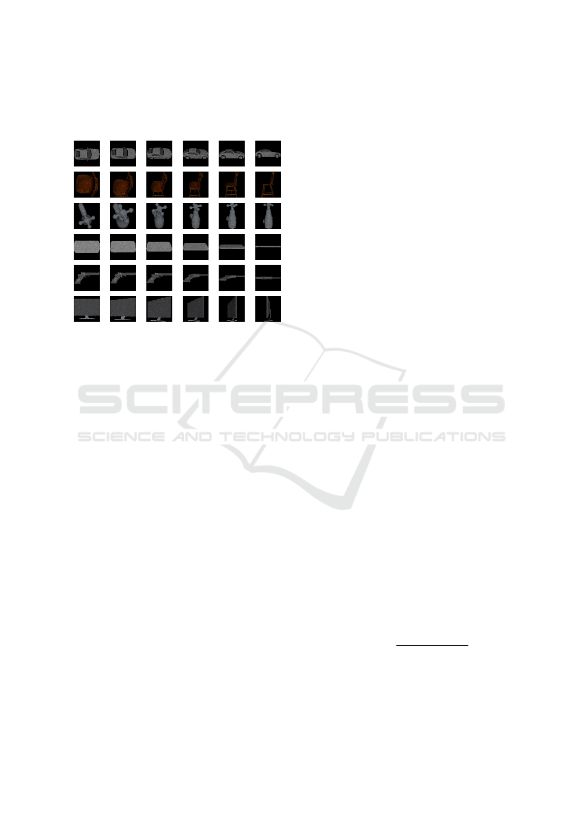
of our method. The dataset consist of objects of six

classes (car, faucet, chair, phone, screen, pistol) and

the models were derived from the ShapeNet dataset

(Chang et al., 2015). The selected objects from the

dataset are presented in Fig. 6. The objects are charac-

terized by different shape, size and visual features. In

a real-world setting it would be an extremely arduous

effort to create an annotated dataset, which fully cov-

ers all objects’ representation in the space of all pos-

sible Euler rotations with varying distance. The cur-

rently available non-synthetic datasets such as YCB

Video (Xiang et al., 2018) and LineMOD (Hinter-

stoisser et al., 2011) provide very detailed images and

Hybrid 6D Object Pose Estimation from the RGB Image

545

annotations of object of different classes but the ob-

jects are not sampled uniformly and some camera an-

gles are omitted due to the manual camera operation.

Figure 6: Representations of objects from our dataset (from

the top row: car, chair, faucet, phone, pistol, screen).

The easiness of creating synthetic sceneries with

predeﬁned conditions suits best the scenario of train-

ing neural networks for big data consumption. We

have therefore rendered multitude of samples for ev-

ery aforementioned object.

The dataset consists of 256 × 256 px RGB images

and binary masks. The camera points from which the

objects have been rendered were laid out uniformly

on a surface of unit sphere. These points have been

also multiplied by random distance factor in order to

achieve representations of varying magnitude and per-

spective. The in-place rotation angle ranged from -60

up to 60 degrees with a step of 3 degrees.

Each object has been rendered with random back-

ground images which have been derived from the Pas-

cal VOC dataset.

2.9 Training the Networks

We trained every module of pose estimation pipeline

independently. The Mask R-CNN network was al-

ready pretrained on the COCO dataset, containing 80

classes. As a next step we ﬁne-tuned the pretrained

network on a smaller dataset of objects.

Training both 4D-NET and 2D-NET was common

when it comes to data preparation stage. It is worth to

mention that the visual centre of bounding box does

not necessarily match the geometrical center of ob-

ject. Moreover, the input data has to be cropped to the

dimensions of 64 × 64px The rectangular bounding

box must be properly transformed to a square shape

with respect to the center position. The Mask R-CNN

does not extract instances perfectly in all cases. For

that reason we shift and scale the bounding boxes, so

that the ﬁnal crops are not matched perfectly. Bound-

ing boxes randomization increases robustness to im-

precisely detected mask through Mask R-CNN.

The 4D-NET was trained with the batch size of

2 and learning rate=0.001. The network was being

trained 12 hours on Nvidia Titan XP before reaching

satisfactory results. The 2D-NET was trained with

the batch size of 5 and with the same learning rate

as the previous network. It turned out that the centre

detection is not challenging and the network provides

close to zero error after one hour of training.

3 RESULTS

3.1 Center Estimation

We have tested the performance of the network for

middle point detection on the test data from our

dataset. The samples provided by the dataset contain

images with binary masks and middle point coordi-

nates of the objects. Therefore we used this informa-

tion to create excerpts using bounding boxes of ran-

domized origin positions and dimensions. The idea

bounding box randomization resembles the case of

inexact instance segmentation of the object extractor.

This approach allowed us to test the robustness of the

network while having only limited data.

The used error metrics for center point estimation

was the Euclidean distance between for both normal-

ized and absolute 2D image coordinates. We use im-

age excerpt coordinates in order to compare the accu-

racy of middle point detection. At the very end the

excerpts are resized to match the dimensions of the

input layer of neural network.

The testing procedure using randomized bounding

boxes always ensures that the object is present in an

image. However, some part the object may be invisi-

ble. We have observed that the network performs very

well given a valid object excerpt. Images presented in

Fig. 7 reﬂect sample predictions produced be the net-

work.

The pixel distance error is represented by follow-

ing equation:

distance

( ˆx − x)

+ ( ˆy − y)

. (8)

The results of the center estimation for each object

from the dataset are presented in Tab. 1. The average

inference error was within 1.72 px for all of the ob-

jects in our dataset. We did not noticed any signiﬁcant

ICINCO 2019 - 16th International Conference on Informatics in Control, Automation and Robotics

546

outliers during the testing phase. The resultant error

exerts only a slight inﬂuence on the ultimately esti-

mated pose. The ﬁnal error derived from the network

for center detection depends linearly on the initial res-

olution of an image except due to the scale factor.

Table 1: Results of the object’s center estimation.

car chair faucet screen phone pistol average

distance

[px] 1.89 1.77 1.07 1.75 1.64 2.17 1.72

distance std

[px] 1.53 1.45 1.06 1.60 1.55 2.10 1.55

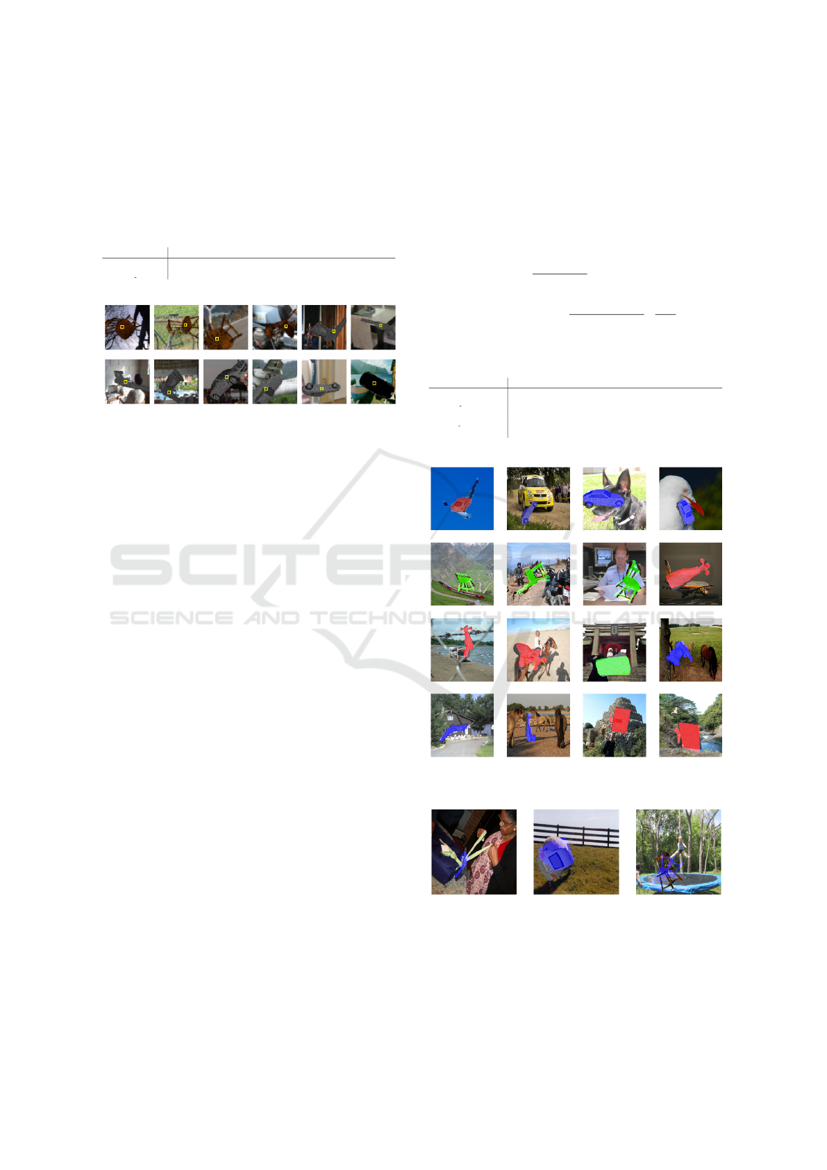
Figure 7: Example results of the object center estimation.

3.2 Pose Estimation

In the case of pose estimation we have tested the

whole pipeline consisting of three neural networks to

evaluate the inference error. The resultant inference

error is inﬂuenced only to a small degree by the cen-

ter detection network. Therefore the ﬁnal pose pre-

diction may be impaired estimated when the 4D-NET

network does not perform well. The input data for

testing procedure were the object representations de-

tected by Mask-RCNN network. We only evaluated

the error metrics for valid detections.

We considered the Euclidean distance error, the

distance between rotation in angle-axis representation

and IoU as the metrics applied for testing the valid-

ity of the method. In order to disregard the distance

disparity among the rendered objects of different size

we normalize the absolute distance error separately

for each label. The results on the pose estimation are

summarized in Tab. 2.

We have established that is possible to retrieve

6D pose based within a tolerable margin using only

color data. The average distance error adds up to 9

cm which is an acceptable result since we use only

cropped and resized color data. The relative distance

can therefore be determined according to the minor

changes of object representation caused by camera

projection. The rotation error lies within a range from

9 to 12 degrees. We noticed that the in-place angle

step used for dataset creation has a major impact on

the rotation error. The more in-place angles are used

for every single camera position, the better rotation

estimation becomes. During the inference stage we

have observed outliers to occur rarely for both dis-

tance and rotation parts. The effectiveness of cen-

ter point estimation allowed to achieve representation

with a high IoU factor as the binary masks overlap

each other to a very large extent in most of the cases.

The normalized distance and rotation errors are

deﬁned by equation (9). We express the rotation dif-

ference between two rotation matrices in degrees:

distance

||T −

T ||

||T ||

· 100%,

rotation

= arccos



R ·



− 1

180

(9)

Table 2: Pose estimation results.

car chair faucet screen phone pistol average

distance

[%] 5.43 6.19 5.87 6.59 7.12 5.57 6.12

distance std

[%] 5.12 5.79 6.27 7.04 7.53 5.23 6.16

rotation

[degrees] 2.83 3.19 3.03 3.76 4.22 3.58 3.43

rotation std

[degrees] 3.21 3.68 3.46 4.15 4.59 4.01 3.85

acc

IoU

[%] 97.2 95.6 96.4 96.1 95.8 96.1 96.4

Figure 8: Example estimated 6D poses compared to the

ground truth data.

Figure 9: Invalid pose predictions. The overlaying projec-

tions does not match silhouettes of the presented objects.

We also visualize the pose error on the image

plane by projecting the estimated object pose on the

RGB image. The example results are presented in

Fig. 8.

Hybrid 6D Object Pose Estimation from the RGB Image

547

In some cases the output of the 4D-NET did not

match the ground truth accurately, as it is shown in

the Fig. 9. We have noticed that the biggest error was

caused by rotation disparity. In most of the cases this

was affected by improper in-place angle prediction,

while the translation inﬂuenced the rotational differ-

ence to a relatively small extent. We have established

that such situations make up 8% of all cases during

testing phase.

3.3 Runtime

The biggest overhead in the computation pipeline is

imposed by the Mask R-CNN network. The infer-

ence time for both 4D-NET and 2D-NET are negli-

gible and they jointly provide a result in 7 millisec-

onds on Nvidia Titan XP. Therefore we can report the

runability at approximately 13-15 frames per second.

The complexity of computation is not inﬂuenced sig-

niﬁcantly for multi-object pose estimation since the

proposed network architectures are quite lightweight.

4 CONCLUSIONS AND FUTURE

WORK

In this paper, we show that the 6D pose estimation

can be split into two smaller sub-problems. First, the

neural network (4D-NET) estimates the camera trans-

lation and in-place rotation with respect to the ob-

ject. At this stage, we assume that the camera axis

goes through the center of the object. Second, the full

3D pose of the camera with respect to the object is

computed using the mathematical model of the cam-

era. The two-stage solution to the object pose esti-

mation allows simplifying the problem in comparison

to end-to-end solutions (Kehl et al., 2017). As a re-

sult, the neural network used for the pose estimation

(4D-NET) can be more compact and computationally

efﬁcient.

To detect the object on the RGB image we use

the Mask R-CNN method (He et al., 2017). The cen-

ter of the detected bounding box does not correspond

with the projection of the object’s center on the image

plane. Thus, we designed the neural network which

estimates the center of the object on the image plane

(2D-NET). Finally, we show results on the publicly

available dataset. The obtained average translation

error is smaller than 7% and the obtained rotation er-

ror is smaller than 5 degrees. It means that we can

precisely and efﬁciently (up to 15 frames per second)

estimate the pose of known objects in the 3D space

using RGB image only.

In the future, we are going to verify the method

in real-world robotics applications. We are going to

use the proposed method to detect and grasp the ob-

jects by the mobile manipulating robot. We also plan

to investigate the accuracy of the proposed method in

real-world scenarios and work on the precision of the

pose estimation.

ACKNOWLEDGEMENTS

This work was supported by the National Centre for

Research and Development (NCBR) through project

LIDER/33/0176/L-8/16/NCBR/2017. We gratefully

acknowledge the support of NVIDIA Corporation

with the donation of the Titan Xp GPU used for this

research.

REFERENCES

Bibby, C. and Reid, I. (2016). Robust Real-Time Visual

Tracking Using Pixel-Wise Posteriors. In Forsyth D.,

Torr P., Z. A., editor, Computer Vision – ECCV 2008.

Lecture Notes in Computer Science, vol. 5303, pages

831–844. Springer, Berlin, Heidelberg.

Brachmann, E., Michel, F., Krull, A., Yang, M. Y.,

Gumhold, S., and Rother, C. (2016). Uncertainty-

Driven 6D Pose Estimation of Objects and Scenes

from a Single RGB Image. In IEEE Conference

on Computer Vision and Pattern Recognition, pages

3364–3372. IEEE.

Chang, A., Funkhouser, T., Guibas, L., Hanrahan, P.,

Huang, Q., Li, Z., Savarese, S., Savva, M., Song, S.,

Su, H., Xiao, J., Yi, L., and Yu, F. (2015). Shapenet:

An information-rich 3D model repository. In arXiv

preprint arXiv:1512.03012.

Do, T.-T., Cai, M., Pham, T., and Reid, I. (2018). Deep-

6DPose: Recovering 6D Object Pose from a Single

RGB Image. In arXiv.

He, K., Gkioxari, G., Doll

ar, P., and Ross, G. (2017). Mask

R-CNN. In IEEE International Conference on Com-

puter Vision, pages 2980–2988. IEEE.

Hinterstoisser, S., Holzer, S., Cagniart, C., Ilic, S., Kono-

lige, K., Navab, N., and Lepetit, V. (2011). Multi-

modal templates for real-time detection of texture-less

objects in heavily cluttered scenes. In IEEE Inter-

national Conference on Computer Vision, pages 858–

865. IEEE.

Hinterstoisser, S., Lepetit, V., Ilic, S., Holzer, S., Bradsky,

G., Konolige, K., and Navab, N. (2012). Model Based

Training, Detection and Pose Estimation of Texture-

Less 3D Objects in Heavily Cluttered Scenes. In et al.,

L. K., editor, Computer Vision – ACCV 2012, Lecture

Notes in Computer Science, vol. 7724, pages 548–562.

Springer, Berlin, Heidelberg.

Hodan, T., Zabulis, X., Lourakis, M., Obdrzalek, S., and

Matas, J. (2015). Detection and Fine 3D Pose Es-

timation of Textureless Objects in RGB-D Images.

ICINCO 2019 - 16th International Conference on Informatics in Control, Automation and Robotics

548

In IEEE/RSJ International Conference on Intelligent

Robots and Systems, pages 4421–4428. IEEE.

Kehl, W., Manhardt, F., Ilic, F. T. S., and Navab, N. (2017).

SSD-6D: Making RGB-Based 3D Detection and 6D

Pose Estimation Great Again. In IEEE International

Conference on Computer Vision (ICCV), pages 1530–

1538. IEEE.

Khoshelham, K. (2011). Accuracy Analysis of Kinect

Depth Data, International Archives of the Photogram-

metry. In Remote Sensing and Spatial Information

Sciences, pages 133–138. IEEE.

Konishi, Y., Hattori, K., and Hashimoto, M. (2018). Real-

Time 6D Object Pose Estimation on CPU. In arXiv.

Liu, W., Anguelov, D., Erhan, D., Szegedy, C., Reed, S., Fu,

C.-Y., and Berg, A. (2016). SSD: Single shot multibox

detector, European Conference on Computer Vision.

In et al., L. B., editor, LNCS vol. 9905, pages 21–37.

Springer.

Prisacariu, V. and Reid, I. (2012). PWP3D: Real-time seg-

mentation and tracking of 3D objects. Int. Journal on

Computer Vision, 98(3):335–354.

Segal, A., Haehnel, D., and Thrun, S. (2009). Generalized-

ICP. In In Robotics: Science and Systems.

Sundermeyer, M., Z.-C, Marton, Durner, M., Brucker, M.,

and Triebel, R. (2018). SSD: Single shot multibox

detector, European Conference on Computer Vision.

In European Conference on Computer Vision, pages

699–715.

Tejani, A., Tang, D., Kouskouridas, R., and Kim, T. (2016).

Latent-Class Hough Forests for 3D Object Detection

and Pose Estimation. In et al., F. D., editor, Computer

Vision – ECCV 2014, Lecture Notes in Computer Sci-

ence, vol. 8694, pages 462–477. Springer, Cham.

Tjaden, H., Schwanecke, H., and Schomer, E. (2016). Real-

Time Monocular Segmentation and Pose Tracking of

Multiple Objects. In Leibe, B., Matas, J., Sebe, N.,

and Welling, M., editors, Computer Vision – ECCV

2016. Lecture Notes in Computer Science, vol. 9908,

pages 423–438. Springer, Cham.

Ulrich, M., Wiedemann, C., and Steger, C. (2012). Combin-

ing Scale-Space and Similarity-Based Aspect Graphs

for Fast 3D Object Recognition. IEEE Transac-

tions on Pattern Analysis and Machine Intelligence,

34(10):1902–1914.

Wang, C., Xu, D., Zhu, Y., Martin-Martin, R., Lu, C., Fei-

Fei, L., and Savarese, S. (2019). DenseFusion: 6D

Object Pose Estimation by Iterative Dense Fusion. In

Computer Vision and Pattern Recognition.

Xiang, Y., Schmidt, T., Narayanan, V., and Fox, D. (2018).

PoseCNN: A Convolutional Neural Network for 6D

Object Pose Estimation in Cluttered Scenes. In

Robotics: Science and Systems.

Hybrid 6D Object Pose Estimation from the RGB Image

549