
Average Modeling of Fly-buck Converter
Denys I. Zaikin
1 a
, Simon L. Mikkelsen
1 b
, Stig Jonasen
1
and Konstantin Sirenko
2
1
Serenergy A/S, Aalborg, Denmark
2
EKTOS-Ukraine LLC, Kharkiv, Ukraine
{dza, slm, sjo}@serenergy.com, ksi@ektos.net
Keywords:
Average Model, Fly-buck, Dc/dc Converter.
Abstract:
This document presents an average macro model for the fly-buck converter. The model can be used for both
large and small signal modeling. Parasitic and lossy components are included in the model, and it is partially
based on a conventional average switch model for a buck stage. For isolated output, the analytic solution of
the average current in a secondary winding is proposed. The presented model is implemented in SPICE, and
simulation results are compared to switching model simulation and experimental data.
1 INTRODUCTION
The fly-buck converter has become popular because
it has several advantages, such as good cross regula-
tion, line transient response, and low EMI, (Fang and
Meng, 2015; Karlsson and Persson, 2017; Gu and
Kshirsagar, 2017; Choudhary, 2015; Nowakowski,
2012). It has a simple design and provides multiple
isolated outputs. A small-signal analytical model for
an ideal fly-buck converter was presented in (Wang
et al., 2017), but the effects of component parasitics
could not be predicted.
The proposed model can be used for both large
and small signal analysis and can be simulated in time
or frequency domains. The difficulty of developing
such a model is that leakage inductance current has a
pulsed shape and cannot be approximated with con-
ventional small ripple approximation, (Erickson and
Maksimovic, 2007). To overcome this issue, the cur-
rent is calculated during the instantaneous switching
period, and small ripple approximation is used for the
transformer’s magnetizing inductance current and ca-
pacitor voltages. The model accounts for the losses
and parasitics of semiconductors and magnetics and
has been implemented as a SPICE subcircuit. The fol-
lowing assumptions were considered: the model cov-
ers two isolated outputs, and the dead-time effect is
negligible.
a
https://orcid.org/0000-0003-4080-5631
b
https://orcid.org/0000-0002-9438-3609
2 MODEL DERIVATION
The fly-buck converter’s basic structure is shown
in Fig. 1. The MOSFETS Q
1
and Q
2
have on-state re-
sistances R
on1
and R
on2
, respectively. The transformer
T
1
has secondary side-related leakage inductance L
s
,
magnetizing inductance L
m
, primary winding resis-
tance R
pri
, secondary winding resistance R
s
, and turns
ratio 1 : n. The diode D
1
is modeled with on-state re-
sistance R
D
and forward bias voltage V
D
. Components
listed above are internal parts of the proposed model.
The input voltage v
in
(t), output voltages v
out1
(t) and
v
out2
(t), and the corresponding load networks (R
1
/C
1
and R
2
/C
2
) are connected externally to the model.
The converter has switching frequency F
sw
= 1/T .
v
in
(t)
Q
1
Q
2
i
in
(t)
1:n
i
L
(t)
L
m
R
pri
v
out1
(t)
+
C
1
R
1
L
s
R
s
i
out1
(t)
R
D
V
D
T
1
D
1
v
out2
(t)
+
C
2
R
2
i
out2
(t)
R
on1
R
on2
Figure 1: Fly-buck converter with two outputs.
The main waveforms are shown in Fig. 2.
The switching period is divided into three parts, and
the first interval d
1
is the time when leakage induc-
tance L
s
resets. The switch Q
1
is on, and the Q
2
is
off. The diode D
1
is forward-biased. The second in-
terval d
2
is the time when the diode D
1
blocks, Q
1
is
on, and Q
2
is off. The third interval d
3
is the time
Zaikin, D., Mikkelsen, S., Jonasen, S. and Sirenko, K.
Average Modeling of Fly-buck Converter.
DOI: 10.5220/0007933703270331
In Proceedings of the 9th International Conference on Simulation and Modeling Methodologies, Technologies and Applications (SIMULTECH 2019), pages 327-331
ISBN: 978-989-758-381-0
Copyright
c
2019 by SCITEPRESS – Science and Technology Publications, Lda. All rights reserved
327
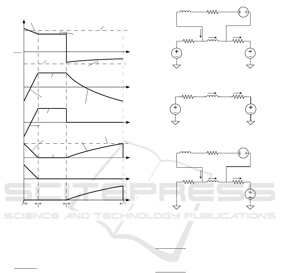
when Q
1
is off, Q
2
is on, and D
1
conducts. The duty
cycle is determined as d = d
1
+ d
2
and 1 − d = d
3
.
i
out1
i
in
i
out2
i
L
-i
out2(d1)
n
i
L
-i
out2(d1)
n
i
L
v
in
-v
out1
-v
out1
d
1
d
2
d
3
i
out2(d1)
i
out2(d3)
i
out2(d2)
=0
i
L
-i
out2(d3)
n
i
out2(d1)
i
out2(d3)
i
L
L
m
di
L
dt
-(i
L
-i
out2(d1)
n)(R
on1
+R
pri
)
-i
L
(R
on1
+R
pri
)
-(i
L
-i
out2(d3)
n)(R
on2
+R
pri
)
max(i
out2
)
T
T0
Figure 2: Waveforms of the fly-buck converter.
States of the converter at each time interval d
1
−d
3
are presented in Fig. 3. Using the small ripple approx-
imation average, voltage across the inductor can be
obtained:
L
m
dhi
L
(t)i
T
dt
= hv
in
(t)i
T
d − hv
out1
(t)i
T
− hi
L
(t)i
T
(R
on1
d + R
on2
(1 − d) + R
pri
)+
hi
out2
(d
1
)
(t)i
T
(R
on1
+ R
pri
)n+
hi
out2
(d
3
)
(t)i
T
(R
on2
+ R
pri
)n, (1)
where hx(t)i
T
represents the average value of x over
the switching period T . The currents i
out2
(d
1
)
(t)
and
i
out2
(d
3
)
(t)
are artificially shown in Fig. 2 separately, so
i
out2
(t) = i
out2
(d
1
)
(t)+i
out2
(d
3
)
(t) due to i
out2
(d
2
)
(t) = 0.
The average values of these currents will be obtained
later.
By using the charge balance approach, the average
currents for C
1
and C
2
can be found:
R
on1
R
pri
L
m
v
in
(t)
v
out1
(t)
L
s
/n
2
(R
s
+R
D
)/n
2
(v
out2
(t)+V
D
)/n
i
L
(t) i
out1
(t)i
out2
(t)*n
d
1
(a)
R
on1
R
pri
L
m
v
in
(t)
v
out1
(t)
i
L
(t)
d
2
(b)
R
on2
R
pri
L
m
v
out1
(t)
L
s
/n
2
(R
s
+R
D
)/n
2
(v
out2
(t)+V
D
)/n
i
L
(t) i
out1
(t)i
out2
(t)*n
d
3
(c)
Figure 3: Equivalent circuits of the converter for different
time intervals.
C
1
d hv
out1
(t)i
T
dt
= −hi
out2
i
T
n − hv
out1
(t)i
T
/R
1
+hi
L
i
T
(2)
C
2
d hv
out2
(t)i
T
dt
= −hv
out2
(t)i
T
/R
2
+ hi
out2
(t)i
T
(3)
The input voltage source’s average current can be ob-
tained as follows:
hi
in
(t)i
T
= hi
L
(t)i
T
d − hi
out2
d1
(t)i
T
n (4)
To build the final model, the average currents
hi
out2
d1
(t)i
T
and hi
out2
d3
(t)i
T
must be obtained. It can
be seen from Fig. 2 that current i
out2
d3
(t) is an ex-
ponential process of magnetizing leakage inductance
L
s
. Fig. 3c can be used to find an analytical solu-
tion for the hi
out2
d3
(t)i
T
average current. The transient
process during one switching period is considered.
Variables i
L
(t), v
out1
(t) and v
out2
(t) can be replaced
with constant sources for one switching period due to
the small ripple approximation. The initial current in
SIMULTECH 2019 - 9th International Conference on Simulation and Modeling Methodologies, Technologies and Applications
328

the L
s
inductor is zero, so a solution for the peak and
average currents can be found:
max(i
out2
)
T
=
E
d3
(t)
R
d3
n
1−e
−
R
d3
n
2
t
o f f
L
s
(5)
hi
out2
d3
(t)i
T
=
E
d3
(t)F
sw
R
d3
n
L
s
1−e
−
R
d3
n
2
t
o f f
L
s
R
d3
n
2
+t
o f f
,
(6)
where R
d3
= R
on2
+R
pri
+(R
s
+ R
D
)/n
2
, t
o f f
= (1−
d)/F
sw
and
E
d3
(t) = hv
out1
(t)i+hi
L
(t)i(R
on2
+R
pri
)−
(hv
out2
(t)i+V
D
)
n
.
A similar approach can be used to find
hi
out2
d1
(t)i
T
’s average current during the d
1
interval.
Fig. 3a represents an equivalent circuit for this inter-
val. Transient process of the leakage inductance reset
is also considered in one particular switching period.
The initial current in the L
s
inductor is max (i
out2
)
T
,
found from (5), and then it resets to zero current.
Thus, the solution is obtained as follows:
hi
out2
d1
(t)i
T
=
E
d3
(t)F
sw
L
s
n
3
R
d1
R
d3
1 − e
−
n
2
t
o f f
R
d3
L
s
+
E
d1
(t)F
sw
L
s
n
3
R
d1
2
ln
1 −
E
d3
(t)R
d1
E
d1
(t)R
d3
1 − e
−
n
2
t
o f f
R
d3
L
s
,
(7)
where E
d1
(t)=E
d3
(t)−hv
in
(t)i−hi
L
(t)i(R
on2
−R
on1
),
R
d1
= R
on1
+ R
pri
+ (R
s
+ R
D
)/n
2
. Using (1)–(3),
the schematic of the fly-buck converter model can be
constructed as shown in Fig. 4. The hi
out2
d1
(t)i
T
and
hi
out2
d3
(t)i
T
currents ((6) and (7)) and realization of
(3) are implemented by the Gd1 and Gd2 arbitrarily
behavior current sources. The E3 source, along with
L1, realizes (1). The G3 source is responsible for (4),
while the G4 source implements (2). The ideal diodes
D1 and D2 improve the convergence of the model by
blocking negative voltages on the second output.
The model has next pins to connect to external cir-
cuits: node ‘Vin’ — input voltage, node ‘Vout1’ —
first output (non-isolated), node ‘Vout2’ — second
output (isolated) and node ‘d’ — duty cycle control
input (0.0...1.0 range). The reference zero potential
for the primary side is connected to the global ‘0’
net, and the secondary side’s ground potential is con-
nected using a GND
SEC pin.
The sub-model netlist can be found in
Fig. 5 and (Zaikin, 2019).
L1
{Lm}
d
dcXFMR
Gd1
Gd3
VALUE={I(Gd1)*n}
G3
VALUE={V(Ed3)-V(Vin)-I(L1)*(Ron2-Ron1)}
Ed1
VALUE={V(Vout1)+I(L1)*(Ron2+Rpri)-(V(Vout2,GND_SEC)+VD)/n}
Ed3
E3
VALUE={-(V(d)*Ron1+(1-V(d))*Ron2+Rpri)*I(L1)+n*(Ron1+Rpri)*I(Gd1)+n*(Ron2+Rpri)*I(Gd3)}
G4
VALUE={(I(Gd1)+I(Gd3))*n}
D1
Dbreak
VALUE={(1-V(d))/Fsw}
Etoff
D2
Dbreak
Vout1Vin
d
Vout2
Ed3 Ed1
1 2
GND_SEC
toff
3
Figure 4: Fly-buck converter average model schematic.
.SUBCKT FLY_BUCK_AVG Vin Vout1 Vout2 GND_SEC d
+PARAMS: Ron1=12m Ron2=12m VD=1.8 RD=0.2 Rs=0.07
+Ls=7.5u Rpri=10m Lm=3.8u n=5 Fsw=100k
.param Rd1={Ron1+Rpri+(Rs+RD)/n**2}
.param Rd3={Ron2+Rpri+(Rs+RD)/n**2}
L1 2 Vout1 {Lm}
Gd1 0 5 VALUE={(V(Ed1)*Fsw*Ls*log(1-(V(Ed3)*Rd1*
+(exp(-(Rd3*n**2*V(toff))/Ls)-1))/(V(Ed1)*Rd3)))/(Rd1**2*
+n**3)+(V(Ed3)*Fsw*Ls*(exp(-(Rd3*n**2*V(toff))/Ls)-1))/
+(Rd1*Rd3*n**3)}
Gd3 0 4 VALUE={(V(Ed3)*Fsw*(v(toff)+(Ls*(exp(-
+(Rd3*n**2*v(toff))/Ls)-1))/(Rd3*n**2)))/(Rd3*n)}
G3 0 Vin VALUE={I(Vd1)*n}
Ed1 Ed1 0 VALUE={V(Ed3)-V(Vin)-I(L1)*(Ron2-Ron1)}
Ed3 Ed3 0 VALUE={V(Vout1)+I(L1)*(Ron2+Rpri)-
+(V(Vout2,0)+VD)/n}
E3 2 1 VALUE={-(V(d)*Ron1+(1-V(d))*Ron2+Rpri)*I(L1)+
+n*(Ron1+Rpri)*I(Vd1)+n*(Ron2+Rpri)*I(Vd3)}
G4 Vout1 0 VALUE={(I(Vd1)+I(Vd3))*n}
D1 0 3 Dbreak
Etoff toff 0 VALUE={(1-V(d))/Fsw}
D2 3 Vout2 Dbreak
Vd3 4 3 0
Vd1 5 3 0
EdcXFMR 6 0 VALUE={V(Vin)*V(d)}
GdcXFMR Vin 0 VALUE={I(VdcXFMR)*V(d)}
RpdcXFRM Vin 0 1MEG
RsdcXFRM 1 7 1u
VdcXFMR 6 7 0
.ends FLY_BUCK_AVG
.model Dbreak D Is=1e-14 Cjo=.1pF Rs=1m N=0.01
Figure 5: The fly-buck converter LTSpice/PSpice sub-
model netlist. Copy-paste is possible from pdf version of
this paper.
AC 1
V1
PULSE({Duty} {Duty-0.1} 10m 10n 10n 5m 12m)
C1
{2*470u*1}
Vin
50
R1
75
Lm
Rpri
Ls
Rs
Ron1
Ron2
Vin
Vout1
Vout2
VDRD
GND_SEC
d
U1
fly_buck_avg
VD=1.8 RD=0.2 Ron1=12m Ron2=12m Fsw={Fsw} Ls={300n*5**2} Rs=0.07 Lm=3.8u Rpri=10m n=5
C3
{0.47u*5}
L1
40µ
C2
{3*180u*8}
R2
100k
R3
25m
R4
35m
Vout1
Vout2
Vin
d
.tran 0 20m 8m 10u uic
.params Pin=1250 Iin=Pin/Vin
+Vout=250 Vin=24
.options plotwinsize=0 method=gear reltol=0.0005 abstol=1u vntol=1m gmin=10p
.params Duty=0.5 Fsw=100k
.include fly_buck_avg.lib
Figure 6: Fly-buck converter simulation setup.
3 RESULTS
The proposed model was simulated and com-
pared to switching modeling, along with proto-
Average Modeling of Fly-buck Converter
329

type measurement. The parameters for simula-
tion and testing were V
D
= 1.8 V, R
D
= 0.2 Ohm
(C3D06060A two in series), R
on1
= R
on2
=12 mOhm
(IPB117N20NFD), F
sw
=100 kHz, Ls =7.5 uH,
Rs=0.07 Ohm, Lm = 3.8 uH, Rpri=10 mOhm, and
n=5. The external circuit contained the input cable’s
40 uH inductance, and capacitance at the input was
7.92 mF (25 mOhm ESR), R
1
=100 kOhm, C
1
=940 uF
(35 mOhm ESR), R
2
=75 Ohm, C
2
=2.35 uF and the in-
put voltage v
in
=50 V. The circuit for simulation and
measurement is shown in Fig. 6. The simulation re-
sults are presented in Fig. 7 and Fig. 8.
Switching model
v
out2
, V
80
90
100
110
120
130
Average model
t, s
0 10
−3
2×10
−3
3×10
−3
4×10
−3
v
out2
, V
80
90
100
110
120
130
Figure 7: Simulation results. The v
out2
step response on
the duty cycle changed from 0.4 to 0.5.
degrees
−300
−250
−200
−150
−100
−50
0
dB
−20
0
40
60
Frequency, Hz
10 100 1000 10
4
10
5
10
6
Magnitude
Phase
Figure 8: Simulation results. The transfer function
ˆv
out2
( f )
ˆ
d( f )
of the output voltage compared to a control.
The setup for testing is shown in Fig. 9. The mea-
surement results are presented in Fig. 10.
Figure 9: Fly-buck converter test setup.
Figure 10: Measurement results. The v
out2
step response on
the duty cycle changed from 0.4 to 0.5.
4 CONCLUSION
The proposed model can be simulated for large and
small signal modeling in time or frequency domains.
The model accounts for parasitics of semiconductors
and magnetics so losses and precise behavior can be
predicted. A listing of the SPICE model was pre-
sented and it can be used for the static and dynamic
behavior analysis of the fly-buck converter.
REFERENCES
Choudhary, V. (2015). Designing isolated rails on the fly
with fly-buck
TM
converters.
Erickson, R. W. and Maksimovic, D. (2007). Fundamentals
of power electronics. Springer Science & Business
Media.
Fang, X. and Meng, Y. (2015). Isolated bias power sup-
ply for igbt gate drives using the fly-buck converter.
SIMULTECH 2019 - 9th International Conference on Simulation and Modeling Methodologies, Technologies and Applications
330

In 2015 IEEE Applied Power Electronics Conference
and Exposition (APEC), pages 2373–2379.
Gu, D. and Kshirsagar, P. (2017). Compact integrated gate
drives and current sensing solution for sic power mod-
ules. In 2017 IEEE Energy Conversion Congress and
Exposition (ECCE), pages 5139–5143.
Karlsson, M. and Persson, O. (2017). Isolated fly-buck con-
verter, switched mode power supply, and method of
measuring a voltage on a secondary side of an isolated
fly-buck converter. US Patent 9,755,532.
Nowakowski, R. (2012). Techniques for implementing a
positive and negative output voltage for industrial and
medical equipment. How2Power Today, pages 1–6.
Wang, W., Lu, D., Chai, Q., Lin, Q., and Cai, F. (2017).
Analysis of fly-buck converter with emphasis on its
cross-regulation. IET Power Electronics, 10(3):292–
301.
Zaikin, D. I. (2019). Files for simulation. https://goo.gl/
EUfctH. Accessed: 2019-03-24.
Average Modeling of Fly-buck Converter
331
