Structure and Parameter Identification of Process Models with Hard
Non-linearities for Industrial Drive Trains by Means of Degenerate
Genetic Programming
Mathias Tantau
1
, Lars Perner
2
, Mark Wielitzka
1
and Tobias Ortmaier
1
1
Institute of Mechatronic Systems, Leibniz University Hanover, Appelstr. 11a, 30165 Hannover, Germany
2
Lenze Automation GmbH, Am Alten Bahnhof 11, D-38122 Braunschweig, Germany
Keywords:
Genetic Programming, Modelling, Simultaneous Identification of Structure and Parameters, Phenomenologi-
cal Models, Backlash, Multiple-mass Resonators.
Abstract:
The derivation of bright-grey box models for electric drives with coupled mechanics, such as stacker cranes,
robots and linear gantries is an important step in control design but often too time-consuming for the ordinary
commissioning process. It requires structure and parameter identification in repeated trial and error loops. In
this paper an automated genetic programming solution is proposed that can cope with various features, includ-
ing highly non-linear mechanics (friction, backlash). The generated state space representation can readily be
used for stability analysis, state control, Kalman filtering, etc. This, however, requires several special rules
in the genetic programming procedure and an automated integration of features into the defining state space
form. Simulations are carried out with industrial data to investigate the performance and robustness.
1 INTRODUCTION
For control design, Kalman filtering, model-based
fault diagnosis (Witczak et al., 2002) in the field of
electric drive trains detailed process models are es-
sential. For these applications it is important that the
models do not only approximate the systems accu-
rately but that they are also physically correct with
interpretable parameters (bright-grey box modelling).
Such phenomenological models (in contrast to black
box models) help to better understand the system of
interest and they allow for advanced techniques from
control theory, such as state control, online parameter
tuning and flatness based control, as they are used in
stacker cranes, robots and linear gantries.
Unfortunately their derivation is very time-
consuming because iteratively different possible mod-
els must be evaluated and then rejected if their com-
plexity is inappropriate or they build on irrelevant
system properties. Genetic programming (GP) of-
fers a solution to the automated identification of
model structures, but classical GP is limited to sim-
ple functions (Koza, 1994). It cannot create the kind
of process models as they are known from electric
drive trains with flexible mechanics, friction or back-
lash. Often they approximate only static functions
(Toropov and Alvarez, 1998).
Extensions to dynamical systems can be found,
often in combination with black-box models that have
a parameter-linear structure (dos Santos Coelho and
Pess
ˆ
oa, 2009). This property facilitates the selection
of important predictors, which can be seen as basic
structure optimization.
If the dynamic models are not linear in parame-
ters, parameters can be included in the form of termi-
nal nodes that are altered by mutations (Winkler et al.,
2004).
In the work of Marenbach et.al. (Marenbach et al.,
1995) the parameter sets of the dynamic transfer func-
tion models are optimized in each step of the GP,
which is time-consuming. In (Gray et al., 1997) a
similar concept with non-linear models like saturation
is presented. The problem remains that the resulting
process models can hardly be interpreted physically
and they are not given in a structured form as required
for example for control design.
The aim of this paper is to derive transparent,
physically motivated process models for electric drive
trains by combining a-priori knowledge with GP
structure identification. The function set is tailored
to the specific properties of electric drives with imper-
fect mechanics. The resulting models are organized in
368
Tantau, M., Perner, L., Wielitzka, M. and Ortmaier, T.
Structure and Parameter Identification of Process Models with Hard Non-linearities for Industrial Drive Trains by Means of Degenerate Genetic Programming.
DOI: 10.5220/0007949003680376
In Proceedings of the 16th International Conference on Informatics in Control, Automation and Robotics (ICINCO 2019), pages 368-376
ISBN: 978-989-758-380-3
Copyright
c
 2019 by SCITEPRESS – Science and Technology Publications, Lda. All rights reserved

the form of state space representations that can be the
starting point for the above mentioned techniques or
for further investigations like controllability and sta-
bility analysis. The intend is that the resulting models
look similar to those designed by an experienced engi-
neer although being created automatically. The struc-
tures are not, however, claimed to be the best possible
way of modelling and equivalent models may exist as
the state space description is per se not unique.
2 PHENOMENOLOGICAL
MODELLING OF ELECTRIC
DRIVES
Structure optimization by GP in this paper means op-
timizing the discrete quantity of different subsections
of the overall process model. These subsections are
also called submodels, associated with known physi-
cal effects as described in the following. In genetic
programming terms they define the function set that
the algorithm can choose from when building the in-
dividuals of the population. When the quantity of a
certain submodel is changed from 0 to 1, it means that
the associated physical effect is now included in the
model. Quantities greater than one are also conceiv-
able, e.g. for simultaneous friction at different loca-
tions.
2.1 Physical Effects
Physical effects, also called properties or features de-
fine the behaviour of the overall model by their com-
pilation. The following list enumerates all the proper-
ties incorporated in the function set of this paper. Fu-
ture extensions are possible, but it is believed that the
given set comprises a reasonably comprehensive se-
lection of typically considered physical effects, while
still maintaining structural output distinguishability
(s.o.d.) (Walter et al., 1984). Although not proven,
the function set is chosen such that s.o.d. should be
respected because for each submodel it is possible to
describe its characteristic, distinct contribution to the
input-output behaviour. Further restrictions of diver-
sity will be introduced in section 3.1.
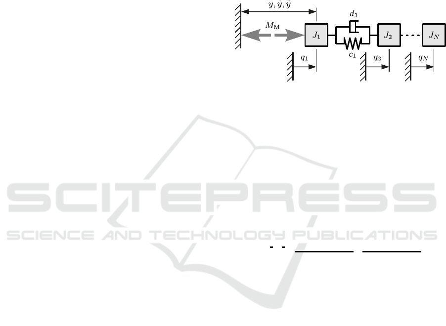
Multiple-mass Systems with Different Numbers of
Masses: Figure 1 is a translational sketch of the
considered class of rotatory multiple mass systems,
showing the angular coordinates q
i
, the moments of
inertia J
i
, the spring constants c
i
and damper constants
d
i
. N ∈ {1, 2,3,4} is the number of masses. The sen-
sor signals q, ˙q and ¨q are strictly bound to the first in-
ertia in this paper, as is the actuator with its torque
M
M
. Other configurations are possible but would
easily lead to ambiguous, indistinguishable transfer
functions and it is believed that this collocated struc-
ture, sometimes called ladder structure can be found
in most electric drive trains anyway, because the col-
location facilitates the control design (Berglund and
Hovland, 2000). The set of estimation parameters is
{
J
i
,c
i
,d
i
}
.
Figure 1: Class of rotatory multiple-mass systems with
motor and position/velocity/acceleration sensor at the first
mass, drawn translational for simplicity.
Multiple mass systems with arbitrary actuator and
sensor positions can be modelled with mass M, damp-
ing D and stiffness matrix C:
M
¨
q + D
˙
q + Cq = F. (1)
Static Friction Model with Three Independent
Components: In agreement with the summands of
the equation
M
F
= − f
v
˙q
i
|{z}
viscous
−tanh( f
tanh
˙q
i
)
h
M
C
+ M
S
e
− ˙q
i
/ ˙q
i,0
i
| {z }
Coulomb and Stribeck
(2)
the friction torque can be divided into three parts: vis-
cous, Coulomb and Stribeck friction (Sch
¨
utte, 2003).
The gain f
tanh
is defined upfront in this study to allow
a stable simulation, leaving only four estimation pa-
rameters:
{
f
v
,M
C
,M
S
, ˙q
i,0
}
. Index i determines the
inertia J
i
with friction.
Gravity: For gravity a constant torque M
G
is added
to the one of the masses so that only the one estima-
tion parameter
{
M
G
}
adds to the overall model.
Backlash: Backlash is included between the first
and second inertia in figure 2. Following the physical
backlash model (Nordin et al., 1997; Zemke, 2012)
the backlash element with a width of 2α is connected
in series with the spring damper element. Coordinate
λ is the position in the backlash gap. When the el-
ement is fully extended, it holds that λ = 0, so the
valid range for λ is −2α ≤ λ ≤ 0. Usually a sym-
metric range is chosen (Zemke, 2012), but here the
deliberately asymmetric range facilitates simulation,
Structure and Parameter Identification of Process Models with Hard Non-linearities for Industrial Drive Trains by Means of Degenerate
Genetic Programming
369

because now the state λ = 0 corresponds to a practi-
cally reproducible initial position.
Figure 2: Backlash between the first and second mass. The
system is considered rotary.
In general, when backlash is added to the spring
damper element with index k between inertias i and
j,
1
the following equation describes the torque that
presses the spring damper element against the adja-
cent inertias:
M
B,k
= c
k
τ
k
+ d
k
˙
τ
k
(3)
with τ
k
= δ
k
− λ
k
,δ
k
= q
i
− q
j
. (4)
Coordinate λ
k
follows the differential equation (k be-
ing omitted)
˙
λ = f
λ
(.) =







max

0,
˙
δ +
c
d
(δ − λ)

for λ = −2α
˙
δ +
c
d
(δ − λ) for − 2α < λ < 0
min

0,
˙
δ +
c
d
(δ − λ)

for λ = 0.
(5)
It represents an integrator with saturation (Nordin
et al., 1997; Zemke, 2012). The only estimation pa-
rameter is
{
α
}
Figure 3 shows the hysteresis loop of the element.
The re-engagement points at the margins of the back-
lash gap may deviate slightly from −2α or 0 if the
spring damper element in preloaded.
Current Control: The current control loop is ap-
proximated by a P
T1
-element. This is commonly done
because the electric constants are much smaller than
the mechanical time constants (Sch
¨
utte, 2003). The
new estimation parameter is the reset time
{
T
1
}
.
Delay Time: Only one external delay is considered.
The transfer function has one parameter
{
T
d
}
in the
case of single-input single-output (SISO) systems:
G
dead
= e
−T
d
s
. (6)
1
Index j is not necessarily i + 1 if spring damper ele-
ments are allowed to be spanned between arbitrary combi-
nations of masses, for example mass 1 and 3.
Figure 3: Hysteresis loop of the spring damper element with
backlash.
2.2 Interchangeable Construction Kit
In order to automate the process of modelling and
structure identification it is necessary to define sub-
models for the physical effects that can be assembled
by an algorithm that has no physical understanding.
The interfaces must be defined in a way that all per-
missible combinations of submodels lead to valid, ex-
ecutable simulation models when combined and no
additional adjustments are required. This is a chal-
lenge because the various submodels are given in dif-
ferent forms (equations of motion, transfer functions,
piecewisely defined functions). Also, the concept
must allow for interchangeable extensions to the func-
tion set defined so far.
As a solution a kind of ”construction kit” mod-
elling in state space form is proposed. Figure 4 shows
the general structure. Matrices A,B,C and D repre-
sent the linear part, while the system function f(x,u)
and output function g(x, u) form the non-linear part
of the model. Time delay is provided for at the input
and output.
Figure 4: State space representation of the construction kit
modelling with linear and non-linear part.
Initially the state space form is empty having no
states. Then the submodels are added as described be-
low, in the given order. The operations do not change
the general shape, but only the content.
Multiple-mass Systems with Different Numbers of
Masses: From M, D and C a linear state space form
ICINCO 2019 - 16th International Conference on Informatics in Control, Automation and Robotics
370

can be derived:
A
Z
=

0
N×N
I
N×N
−M
−1
C −M
−1
D

, (7)
B
Z
=

0
N×N
M
−1

, (8)
C
Z
=

I
2N×2N

0
N×N
I
N×N

A
Z

, (9)
D
Z
=

0
2N×N

0
N×N
I
N×N

B
Z

, (10)
The symbols I and 0 represent unity matrix or zero
matrix, respectively. The input of the resulting MIMO
system is a vector of torques, one for each inertia. The
output is a vector composed of 3N elements for posi-
tion, velocity and acceleration (q,
˙
q,
¨
q)
T
. Later, the
actual actuator and sensor positions will be defined.
Static Friction Model with Three Independent
Components: The friction torque M
F
introduced
above acts as a non-linear state feedback, which
doesn’t exist in the state space form from figure 4. It
must be calculated into a system function and added
to f(x,u):
f(x,u) := f(x, u) + B
Z


0
i−1×1
M
F
( ˙q
i
)
0
N−i×1


. (11)
Gravity: Gravity can be interpreted as a non-linear
feedback at the input i, similar to friction. The only
difference is that the gravity torque is independent of
the system states.
Backlash: The physical backlash model is more
complicated to integrate because it affects the number
of states. Again the case is considered that backlash
is added to the spring damper element k that connects
inertia i with inertia j. The procedure follows five
steps:
1. State λ
k
is added to the state space form without
any connections to inputs, states and outputs.
2. In order to simplify the calculations only a subset
of the state space form is further addressed, de-
fined by the reduced inputs, states and outputs,
and correspondingly A
red
, B
red
, C
red
, D
red
, f
red
,
g
red
:
u
red
=
{}
, (12)
x
red
=

q
i
,q
j
,λ
k
, ˙q
i
, ˙q
j

, (13)
y
red
=

¨q
i
, ¨q
j

. (14)
By this means the next steps are independent of
all properties that may have been added before.
3. This step incorporates the linear spring feedback
at state λ
k
. To do so, a matrix A
add
of appropri-
ate size is added to the system matrix A
red
. It
has only zeros, except for A
add4,3
= A
red4,2
and
A
add5,3
= −A
red5,1
. By reading the entries of the
system matrix the resulting spring damper ele-
ment with backlash will have the same stiffness
constant as the original spring damper element.
4. The non-linear system function
f
add
= (0, 0, f
λ
,A
red4,5
f
λ
,−A
red5,4
f
λ
)
T
(15)
is added to the previously defined subset of the
system function. The third element f
λ
is the non-
linear equation (5). The last two entries incor-
porate the damping feedback. Because
˙
λ
k
is not
available as a state, its system function f
λ
is used
instead.
5. Finally the output matrix and output function must
be updated because system matrix and system
function have changed: C
red
= A
red4−5
, g
red
=
f
red4−5
. The notation means that rows 4 and 5 are
used.
The procedure can be repeated, adding backlash also
to other spring damper elements.
Input and Output Selection Matrix: Next, the
sensor and actuator positions are defined. The actu-
ators are defined by the input selection matrix with N
rows and as many columns as there are actuators. It
is multiplied at the input of the state space represen-
tation. The sensors are defined by an output multipli-
cation with the output selection matrix with 3N rows
and as many columns as there are sensors. Input and
output selection matrix are always required and they
are therefore not explicitly included in the GP func-
tion set.
Current Control: Our approximation as a P
T1
ele-
ment can be regarded as a series connection from the
left. The linear state space form of the current control
is given by
A
L
= −1/T
1
, B
L
= 1/T
1
, C
L
= 1, D
L
= 0.
(16)
Delay Time: In figure 4 the two blocks on the right
and on the left are assigned to delay time. In the SISO
case it is irrelevant which of them is actually used. For
time-domain simulation the signal is resampled gen-
erating intermediate steps by means of linear interpo-
lation.
Structure and Parameter Identification of Process Models with Hard Non-linearities for Industrial Drive Trains by Means of Degenerate
Genetic Programming
371

3 GENETIC PROGRAMMING
The aim is to identify the structure and parameters of
a given reference system, of which the time domain
response to an excitation has been measured previ-
ously. The reference system is either a testbed or only
another simulation model. With the previously de-
fined submodels the process can be formalized as ge-
netic programming. Submodels from the function set
can be included or excluded automatically and no fur-
ther adjustments are necessary. For each constructed
simulation model the estimation parameters are iden-
tified with a global parameter optimization algorithm,
before the fitness of the individual is evaluated.
3.1 Procedure of Genetic Programming
When contrasted with classical genetic programming
as described for example in (Koza, 1994), a few spe-
cial cases must be considered making this genetic pro-
gramming degenerate. Usually the order of the nodes
in a GP tree is part of the function definition and the
output of one node is the input of another node. That
is different here: Each node is assigned a model type
and the number of nodes with a certain model type de-
fines the multiplicity of this submodel. Connections
between nodes do not represent the flow of informa-
tion but merrily the genetic connection as bases on a
chromosome, which is relevant for the mechanisms of
evolution, see below. The number of branches origi-
nating from one node is chosen randomly.
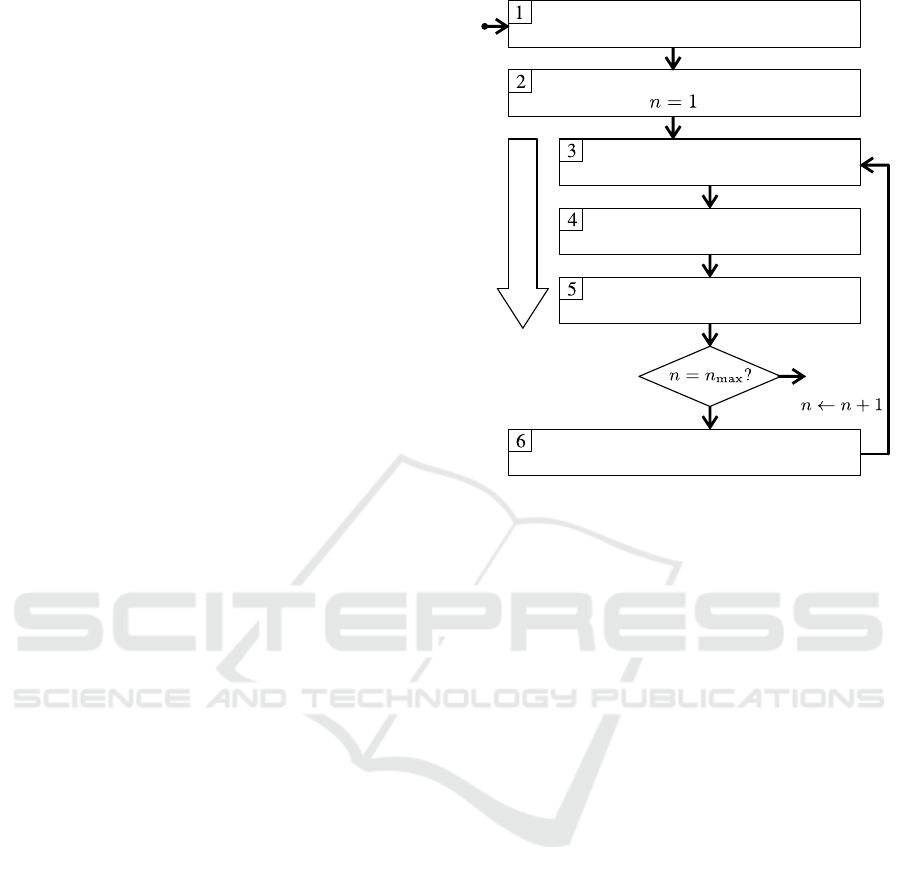
The procedure is sketched in figure 5. In step 1
the function set is defined and for all estimation pa-
rameters included in the function set lower bound and
upper bound are set. For the function set see section
2. It is further restricted according to these rules:
• There is only one sensor and one actuator at iner-
tia 1.
• Only mass 1 may be subject to gravity and fric-
tion.
• Backlash occurs only between inertias 1 and 2.
These restrictions have been set in order to keep the
construction rules, see below, manageable, and also to
avoid the occurrence of practically indistinguishable
models. In this first step the user has the opportunity
to integrate prior knowledge by further restricting the
function set and by defining application-specified pa-
rameter ranges.
Step 2 defines the initial population by creating
trees with a randomly chosen number of nodes, rang-
ing from 1 to the maximal possible number of sub-
models that leads to a model with all features enabled.
For each node a model type is chosen by random from
Definition of the function set and
parameter ranges
Creation of a random initial population
Building the simulation target
including discretisation
Identification of the model
parameters in time domain
Calculation of the fitness
End
Genetic operations
For each individual
Yes
No
Figure 5: Flowchart of genetic programming.
a subset of the function set that leads to a syntactically
valid model following the construction rules, see be-
low. This process may be terminated early if the re-
quired number of nodes cannot be reached because
the features exclude each other, e.g. a one-mass sys-
tem cannot have backlash between masses. The ori-
gin of each new node is chosen randomly from one
of the existing nodes. Initial parameters are chosen
randomly within the permissible range.
In step 3 the time domain identification in Matlab
is prepared by converting the state space form into
system function and output function:
˙
x = f
sys
(x,u) = Ax + Bu + f(x,u) (17)
y = f
sys
(x,u) = Cx + Du + g(x,u). (18)
Function f
out
is discretised using Euler method and
the delay time in included by means of linear interpo-
lation.
In step 4 the set of estimation parameters of
each model is identified by repeatedly simulating the
model for different parameter sets. Penalty for the op-
timizer is the quadratic error between the output of the
simulation model and the reference model. The opti-
mizer patternsearch is used because it considers ini-
tial values of parameters as well as parameter bounds,
while being robust to local minima. The initial sys-
tem states are set corresponding to the real states of
the testbed.
Step 5 is the calculation of fitness under consider-
ICINCO 2019 - 16th International Conference on Informatics in Control, Automation and Robotics
372

ation of the model complexity:
f itness =
1
RSS · (1 + k
P
d)
, (19)
where d is the number of estimation parameters, RSS
is the residual sum of squares of the error in time do-
main. With k
P
the trade-off between model complex-
ity and accuracy can be adjusted. Here, it has been
set to 2. Information criteria could be used instead,
but they require knowledge of the measurement noise
(James et al., 2013) and experiments have shown that
they lead to rather high model complexities if the
number of samples is large.
The genetic operations of step 6 are explained in
the following section.
3.2 Genetic Operations
In step 6 of figure 5 genetic operations are performed
on the current population to create the offspring. First,
new individuals are created by means of recombi-
nation, also called crossover or also by means of
cloning. The percentage that an individual is just
cloned from the parent population is p
clone
. So the
number of cloned individuals stems from a Binomial
distribution N
clone
∼ B(n
P
, p
clone
) with n
P
the size of
the population. A total of N
P
− N
clone
individuals is
generated by means of recombination: The first par-
ent is copied up to a randomly chosen node. The
branch behind this node is replaced by a branch of
the second parent, the origin of which is also chosen
randomly. Each new node is not added but dropped if
a construction rule would be violated by adding it. At
the end a node with a one-mass system is added if no
multiple-mass system exists.
Choosing a parent either for cloning or for repro-
duction is done via Roulette Wheel Selection based on
the fitness, see (Nelles, 2001).
After the new population has been created, differ-
ent kinds of mutations are performed with a certain
probability:
• Point Mutation: One randomly chosen node is
assigned a random, new model type that satisfies
the construction rules. The new estimation param-
eters are defined randomly within the permissible
range.
• Insertion Mutation: A node is added, if possi-
ble, originating from a randomly chosen existing
node. Its model type is random but satisfies the
construction rules.
• Deletion Mutation: A randomly chosen node is
deleted, again only if the construction rules are
respected by the operation.
• Chromosome Mutation: In this mutation a node
is also chosen randomly, but the mutation is not
limited to the one node. Instead, the node and the
whole branch originating from it is replaced by
a new, randomly grown branch that satisfies the
construction rules. The size of the resulting tree
is set randomly, but not less than the original tree
without the new branch. This kind of mutation is
inspired by (Koza, 1994).
Construction Rules. Whenever a genetic operation
is performed or when the initial population is created,
the construction rules must be considered:
• Each model can be included a minimum of 0 times
and a maximum of 1 time.
• Exactly one model of the general type ’multiple-
mass system’ must be included in all individuals.
• The model type ’one-mass system’ is mutually ex-
clusive with the model type ’backlash’.
It is believed that the mutations play an important
role in the parameter identification. When nodes are
copied from the parent population in cloning or re-
combination, the current parameter estimates are also
copied and used as a starting point for the optimiza-
tion in the next generation. As a consequence, previ-
ously found good solutions are passed on to the next
generation shortening optimization time and preserv-
ing good solutions. However, the drawback is that the
optimizer is subject to premature convergence due to
this procedure. When new, random parameters are
reintroduced by the mutations, local minima can be
escaped. The same is true for the structure optimiza-
tion.
4 SIMULATION RESULTS
A reference model is simulated and its output is used
instead of real measurements. The reference model
is a 2-mass resonating system with all three friction
components but no gravity, current control or delay
time, no noise. The excitation for the reference model
and the optimization models is a torque signal that
would lead to a standard industrial jerk-limited re-
versing motion if applied to a single moving mass,
see figure 6.
As output the velocity at mass 1 is used. The lower
and upper bounds of the estimation parameters are set
to 50 %, resp. 200 % of the assumed values. Only the
gravity torque has a range centred around 0 because
gravity is allowed to be both positive and negative.
The GP algorithm is run for 20 generations with 6 in-
dividuals. For the parameter optimization a maximum
Structure and Parameter Identification of Process Models with Hard Non-linearities for Industrial Drive Trains by Means of Degenerate
Genetic Programming
373

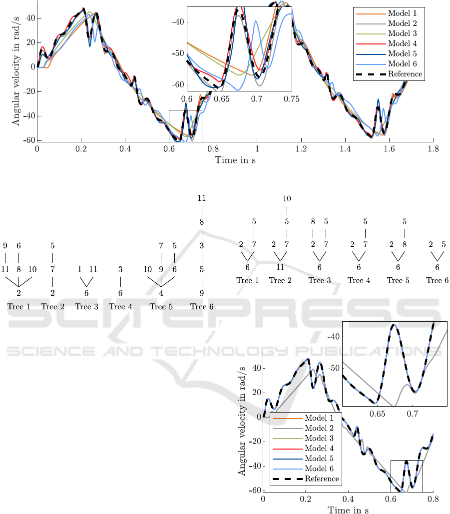
Figure 6: Output velocities of the 6 models of the initial population.
Figure 7: Initial population. 1: 1-mass system, 2: 2-mass
system, 3: 3-mass system, 4: 4-mass system, 5: Coulomb
friction, 6: viscous friction, 7: Stribeck friction, 8: gravity,
9: backlash, 10: current control, 11: delay time. The order
has no meaning.
of 500 iterations is allowed for each individual of each
generation.
Figure 7 shows the six trees of the initial popu-
lation. Model types are represented by numbers, see
figure description.
With this initial population the outputs in figure
6 have been retrieved after performing steps 3 and 4
in figure 5. It can be seen that some of the models fit
better than others. In general, the differences from the
reference model are obvious.
After 8 generations a population as in figure 8 has
evolved, which includes the correct model (2,5,6,7)
two times. The remaining four individuals look rela-
tively similar which indicates that they have a com-
mon parent and mutations have caused the differ-
ences.
Figure 9 shows the outputs of the 6 models from
figure 8. Most of these models are so close to the ref-
erence model trajectory that they are not distinguish-
able. Only model 2 with delay time, behaves clearly
distinct.
Although the correct model has been found in gen-
Figure 8: Generation 8. The numbers stand for the model
types, see figure 7.
Figure 9: Output velocities of the 6 models of the eighth
population. For space reasons only the first 0.8 s are dis-
played.
eration 8, all 20 generations are performed, because
in a real scenario the optimal model is unknown.
Repeating the simulation shows that sometimes the
resulting model has extra gravity or more than two
masses. In this case the fitness is inferior but visually
the trajectories can hardly be distinguished.
ICINCO 2019 - 16th International Conference on Informatics in Control, Automation and Robotics
374

What has been shown for a 2-mass system with
friction is also applicable to other compilations of the
above candidate functions. The success depends on
the estimation parameter ranges, the excitation trajec-
tory and on the reference model parameters. E.g. a
delay time of 50ms can be detected more easily that a
delay time of 1ms.
5 DISCUSSION
Although the success is remarkable given the short
excitation of ≈ 2 s and the difficulty of deriving
knowledge about the inner structure from an obser-
vation of the input-output behaviour, the results of the
method should be interpreted with caution. Clearly,
the distinguishability of structures depends on many
factors and it has not been proven that it is given for all
candidate models considered here. In fact, the simula-
tions have shown that repetitions can lead to different
results, which may also be enforced by the inherently
random nature of the optimization. As a mitigation,
the small numbers of 20 iterations and 6 individuals
could by increased. Also, an explicit separation into
training and test data could improve the reliability of
the result. But still, the veracity of the output models
should be reviewed cautiously before any conclusions
are drawn.
Another limitation of the approach is that it incor-
porates only little prior knowledge and accordingly
the resulting models can only be relatively simple.
Application-specific knowledge about special effects,
such as position dependencies, non-linear springs etc.
cannot readily be included. As a consequence, several
restrictions of diversity had to be introduced such as
the restriction to one external delay, or to collocated
multiple-mass systems.
It must however be stressed that the intend of this
paper was not to identify a unique state space descrip-
tion, which would be impossible, but only a model in
a commonly acknowledged form with physically in-
terpretable parameters. On that basis, the results can
be seen as a success.
The GP algorithm described here is unusual in the
way that the exact order of notes has no influence on
the resulting model. So the benefit of the tree struc-
ture over a simple list of functions is not fully uti-
lized. But this is also the case in other applications
of genetic programming, when e.g. the order of mul-
tiplication or summation elements is ”optimized” al-
though it is irrelevant. The tree structure still develops
a merit when mutations or crossover are performed.
6 CONCLUSIONS AND FUTURE
WORKS
6.1 Conclusions
Dynamic structure identification by means of genetic
programming has been extended to models of elec-
tric drives with hard non-linearities. The generated
state space representation can readily be used for con-
trol design and analysis. Its parsimony is optimized,
i.e. the number of estimation parameters is minimized
while maintaining accuracy. The concept can be ex-
tended interchangeably.
Because of the intricate engagement of the various
kinds of submodels into the overall model several ad-
ditional grammar rules must be incorporated into the
GP algorithm. Successful operation has been shown
exemplarily but cannot be guaranteed because of the
stochastic nature of the algorithm.
6.2 Future Works
Future works include the generalisation to other sen-
sor and actuator configurations and the inclusion
of branching multiple-mass systems instead of the
purely linear ladder structure. The structure identi-
fication could be carried out on the basis of adding
and removing single spring-damper elements. Fur-
thermore, a systematic tuning of the excitation signal
to excite all parameters equally well is conceivable.
ACKNOWLEDGEMENTS
This work was sponsored by the German
Forschungsvereinigung Antriebstechnik e.V. (FVA).
REFERENCES
Berglund, E. and Hovland, G. E. (2000). Automatic elas-
ticity tuning of industrial robot manipulators. In Pro-
ceedings of the 39th Conference on Decision and Con-
trol, volume 5, pages 5091–5096. IEEE.
dos Santos Coelho, L. and Pess
ˆ
oa, M. W. (2009). Nonlinear
model identification of an experimental ball-and-tube
system using a genetic programming approach. Me-
chanical Systems and Signal Processing, 23(5):1434–
1446.
Gray, G. J., Weinbrenner, T., Murray-Smith, D. J., Li, Y.,
and Sharman, K. C. (1997). Issues in nonlinear model
structure identification using genetic programming. In
Genetic Algorithms in Engineering Systems: Innova-
tions and Applications, volume 446, pages 308–313.
Structure and Parameter Identification of Process Models with Hard Non-linearities for Industrial Drive Trains by Means of Degenerate
Genetic Programming
375

James, G., Witten, D., Hastie, T., and Tibshirani, R. (2013).
An introduction to statistical learning. Springer.
Koza, J. R. (1994). Genetic programming II, volume 17.
MIT press Cambridge, MA.
Marenbach, P., Bettenhausen, K. D., and Cuno, B.
(1995). Selbstorganisierende Generierung strukturi-
erter Prozeßmodelle. at-Automatisierungstechnik,
43(6):277–288.
Nelles, O. (2001). Nonlinear system identification: from
classical approaches to neural networks and fuzzy
models. Springer-Verlag, Berlin.
Nordin, M., Galic’, J., and Gutman, P.-O. (1997). New
models for backlash and gear play. International
journal of adaptive control and signal processing,
11(1):49–63.
Sch
¨
utte, F. (2003). Automatisierte Reglerinbetriebnahme
f
¨
ur elektrische Antriebe mit schwingungsf
¨
ahiger
Mechanik. Shaker.
Toropov, V. and Alvarez, L. (1998). Approximation model
building for design optimization using genetic pro-
gramming methodology. In 7th Symposium on Mul-
tidisciplinary Analysis and Optimization, pages 490–
498.
Walter, E., Lecourtier, Y., and Happel, J. (1984). On
the structural output distinguishability of parametric
models, and its relations with structural identifiability.
IEEE Transactions on Automatic Control, 29(1):56–
57.
Winkler, S., Affenzeller, M., and Wagner, S. (2004). Iden-
tifiying nonlinear model structures using genetic pro-
gramming techniques. Citeseer.
Witczak, M., Obuchowicz, A., and Korbicz, J. (2002). Ge-
netic programming based approaches to identification
and fault diagnosis of non-linear dynamic systems. In-
ternational Journal of Control, 75(13):1012–1031.
Zemke, S. (2012). Analyse und modellbasierte Regelung
von Ruckelschwingungen im Antriebsstrang von
Kraftfahrzeugen. PhD thesis, Leibniz Universit
¨
at
Hannover.
ICINCO 2019 - 16th International Conference on Informatics in Control, Automation and Robotics
376