
Research and Development of High Performance Finite Element for
Large Scale Acoustic Analysis Method
E. Takaoka
a
, Y. Murakami and A. Takei
b
Faculty of Engineering, University of Miyazaki, Miyazaki, Japan
Keywords: Finite Element Method, Acoustic Analysis, Iterative Domain Decomposition Method, High-order Elements.
Abstract: In recent years, numerical methods such as the finite element method are developed for sound field prediction
of architectural spaces. However, large-scale analysis is often necessary because of the larger domains and
the higher frequencies that we deal with in engineering applications. Therefore, we often only consider larger
domains at low frequencies or high frequencies in smaller domains. In this paper, the iterative domain
decomposition method (IDDM) is applied to solve transient and steady-state acoustic problems. By applying
the IDDM, the effectiveness of the large-scale acoustic analysis can be shown. In addition, the results of
introducing high-order elements into the analysis are shown.
1 INTRODUCTION
Prediction of acoustic performance is important for
the design of concert halls (Otsuru, 2002). As
representative examples of the prediction, there are
scale model experiments and computer simulations.
Experiments have been used for a long time in many
fields and are applied to visualization and audibility.
However, they take a lot of time and are expensive to
run. On the other hand, computer simulations can
develop models in the virtual space which are a lot
less expensive than experiments. However, due to the
larger problems considered and the increased
frequencies, the scale of models must also be
increased. Hence, large scale analysis is required.
So far, acoustic analysis methods using the finite
difference time-domain (FDTD) (Sendo, 2002), the
boundary element method (BEM) (Sakuma, 2009),
and the finite element method (FEM) (Okuzono,
2010) have been developed. In the FDTD method,
mesh division is performed using a structured grid.
Therefore, analysis with complicated shapes can be
problematic and application to the analysis of
architectural space is difficult. In the boundary
element method, the boundary of the analyzed region
is divided into elements and analyzed. The method
leads to dense matrices which requires a large amount
of memory. On the other hand, the finite element
a
https://orcid.org/0000-0002-5932-2093
b
https://orcid.org/0000-0001-9014-8727
method can use unstructured mesh grids and can deal
with complex shapes. For these reasons, an acoustic
analysis using the finite element method is developed.
One of the problems of the finite element method
is that the scale of the analysis increases with the
increased frequency. The accuracy of the finite
element method improves as the number of divisions
with respect to the wavelength, increases. As the
frequency increases, the wavelength decreases, and
the number of elements required to obtain sufficient
resolution increases (Urata, 2004). For this reason,
there is a limitation on the wavelengths that can be
analyzed with the finite element method. From such
a background, it is necessary to develop a method
capable of high-accuracy analysis while reducing the
number of elements necessary for analysis, and a
method capable of large-scale analysis. In this study,
by introducing the high-performance finite element,
we aim to reduce the number of elements and develop
the technology corresponding to the expansion of the
analysis domain and the increased frequency.
A parallel finite element steady-state acoustic
analysis method applying the iterative domain
decomposition method (IDDM) as a parallelization
method is proposed. The method have been tested and
shown to perform the steady analysis with a
maximum error of about 1.4 [%] compared to a
reference solution in a benchmark problem
Takaoka, E., Murakami, Y. and Takei, A.
Research and Development of High Performance Finite Element for Large Scale Acoustic Analysis Method.
DOI: 10.5220/0007954403530359
In Proceedings of the 9th International Conference on Simulation and Modeling Methodologies, Technologies and Applications (SIMULTECH 2019), pages 353-359
ISBN: 978-989-758-381-0
Copyright
c
2019 by SCITEPRESS – Science and Technology Publications, Lda. All rights reserved
353

(Murakami, 2019). This has enabled large-scale
calculations with high accuracy as a numerical
acoustic analysis method in steady problems.
In this paper, a transient acoustic analysis method
is developed using time domain parallel finite
element method based on this parallelization method.
We report here that this method has sufficient
accuracy in a benchmark problem and that analysis is
also possible in real environment applications such as
a live house.
2 FORMULATION
2.1 Helmholtz Equation
Let us consider a 3D region with a boundary and a
region inside the boundary. The wave equation for
the velocity potential in the sound field is expressed
by the following equation.
(1)
Where is the velocity potential, [m/s] is the
velocity of sound, and is the distribution function of
a sound source.
Considering a steady-state problem Eq. (2) can be
reduced to the Helmholtz equation (Eq. (3)).
(2)
(3)
Where is the imaginary number, and is the
angular frequency. The sound pressure can be
calculated by the following equation using an
imaginary number j, and medium density [
]
after calculating the velocity potential .
(4)
2.2 Finite Element Formulation
To derive a weak form, the Galerkin method is
applied to Eq. (3). Finite element approximation and
discretization gives the following equation.
(5)
Where [ ] is a matrix, { } is a vector. Now, let the
element matrix of Eq. (5) be []
e
, []
e
, []
e
. When
the shape function and its transpose
are
used, they are expressed as the following equations.
(6)
Where []
e
and []
e
are volume integrals, and []
e
, is a surface integral to the sound absorbing boundary
surface, while
is a specific acoustic impedance.
Matrices [] and [] are symmetric sparse matrices.
Matrix [] has a complex impedance. Therefore, the
entire coefficient matrix is a complex symmetric
matrix.
2.3 Time Domain Problem
To convert to time domain representation, Inverse
Fourier transform is applied to Eq. (5). Thus the
following equation is achieved
(7)
Where,
and
are first-order and second-order
derivatives related to time.
To solve the velocity potential
in the time
domain problem, linear acceleration is applied in the
time dimension of Eq. (8). It is assumed that velocity
potentials
,
and
are known at a time .
Applying the Newmark method (AIJ, 2011),
and
are used in the time stepping form to
can be approximated in the form of the following
equations.
(8)
(9)
From Eq. (7) to (9), the simultaneous linear equation
is obtained.
(10)
Where,
SIMULTECH 2019 - 9th International Conference on Simulation and Modeling Methodologies, Technologies and Applications
354

(11)
From Eq. (8) to (10), the solutions of
and
can be obtained.
The velocity potential of the second derivative of
the unknown can be obtained using the iterative
method of Conjugate Orthogonal Conjugate Gradient
(COCG) for the derived Eq. (11). The solution of the
time domain problem is obtained by repeating these
calculations step by step.
3 PARALLELIZATION
3.1 Interface Problem
In this research, the IDDM is applied as a
parallelization method. This is known as a method
that can solve large-scale simultaneous linear system
of equations efficiently. The procedure of the IDDM
is shown below:
(1). The analysis area is divided into an arbitrary
number of areas (partial areas).
(2). Perform finite element analysis for using
iterative calculation of the interface problem in
between these areas.
(3). With the end of the iterative calculations, obtain
the solution of the whole analysis area.
The simultaneous linear system of equations to be
solved is
(12)
Where, is the coefficient matrix, is the unknown
vector and is the known vector. With the smallest
unit as an element, the analysis area is divided such
that there is no overlap.
(13)
When the domain decomposition method is applied
with
degrees of freedom newly generated on the
boundaries between the regions, and
degrees of
freedom generated on the partial areas, the following
equations are obtained.
(14)
Where,
is a 0-1 matrix that limits
to the
internal degrees of freedom of the partial area. Eq.
(14) leads to the following equations:
,
(15)
(16)
Where,
is the right hand vector for
, and
is the inverse of
. Eq. (16) is the
interface problem (Ogino, 2016) which represents a
connection between areas in the domain
decomposition method.
3.2 IDDM
IDDM is a method to obtain the degrees of freedom
for nodes inside partial areas contained in DDM
iteratively.
In this research, COCG method is applied as an
iterative solution method of IDDM. Where is a
convergence determination value and
is 2-norm.
Figure 1 shows COCG method algorithm for interface
problem.
In (I) and (II) shown in Figure 1, there is a need
for a vector product operation of the Schur
complement matrix. The construction of this matrix
involves a lot of calculations. Therefore, as shown in
Figure 1, calculations are performed by substituting
the finite element method calculation of the partial
area.
The finite element method calculations are
performed for each partial area in each step of the
iterative solution of the interface problem. Therefore,
high parallelism can be expected because it can be
calculated independently.
Research and Development of High Performance Finite Element for Large Scale Acoustic Analysis Method
355
Choose
................................................. (I)
For n=0, 1, 2, ......
............................................................ (II)
IF
<
, break
End For
(Ⅰ) In each subdomain
Compute
by
(Ⅱ) In each subdomain
Compute
by
Figure 1: COCG method algorithm for IDDM.
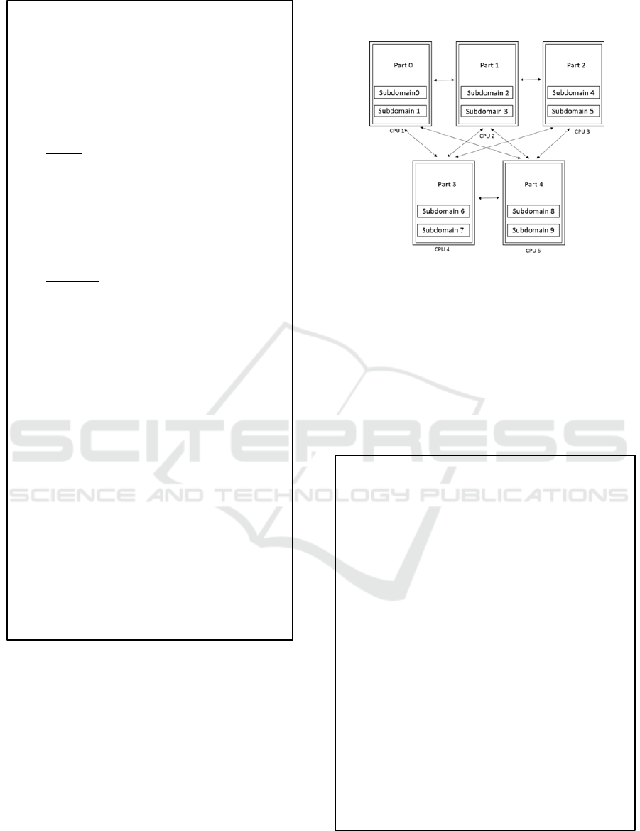
3.3 HDDM
The hierarchical domain decomposition method
(HDDM) is a DDM having a 2-step hierarchy in
which the entire analysis area is first divided into an
arbitrary number of parts, and then divided into
multiple subdomains (Takei, 2010). HDDM is a
method of allocating divided parts to 1 process or 1
thread, performing internal finite element analysis at
each step of the iterative solution method of the
interface problem, and obtain a solution of the whole
analysis area.
The assignment to each computation node of this
method is shown in Figure 2.
Figure 2: Assignment of HDDM to each compute node.
3.4 BDD Pre-processing
The balancing domain decomposition (BDD) pre-
processing is based on the multigrid method, and can
greatly improve the convergence of the interface
problem (Mandel, 1993). The algorithm of BDD pre-
processing is shown in Figure 3. This figure shows
finding
for the residual obtained in each
step of the COCG method.
Step 1 :
is calculated
Step 2:
is calculated
Step 3: Solve the local problem in each region.
Step 4:
is calculated
Step 5: z is calculated
Figure 3: Algorithm of BDD pre-processing.
SIMULTECH 2019 - 9th International Conference on Simulation and Modeling Methodologies, Technologies and Applications
356
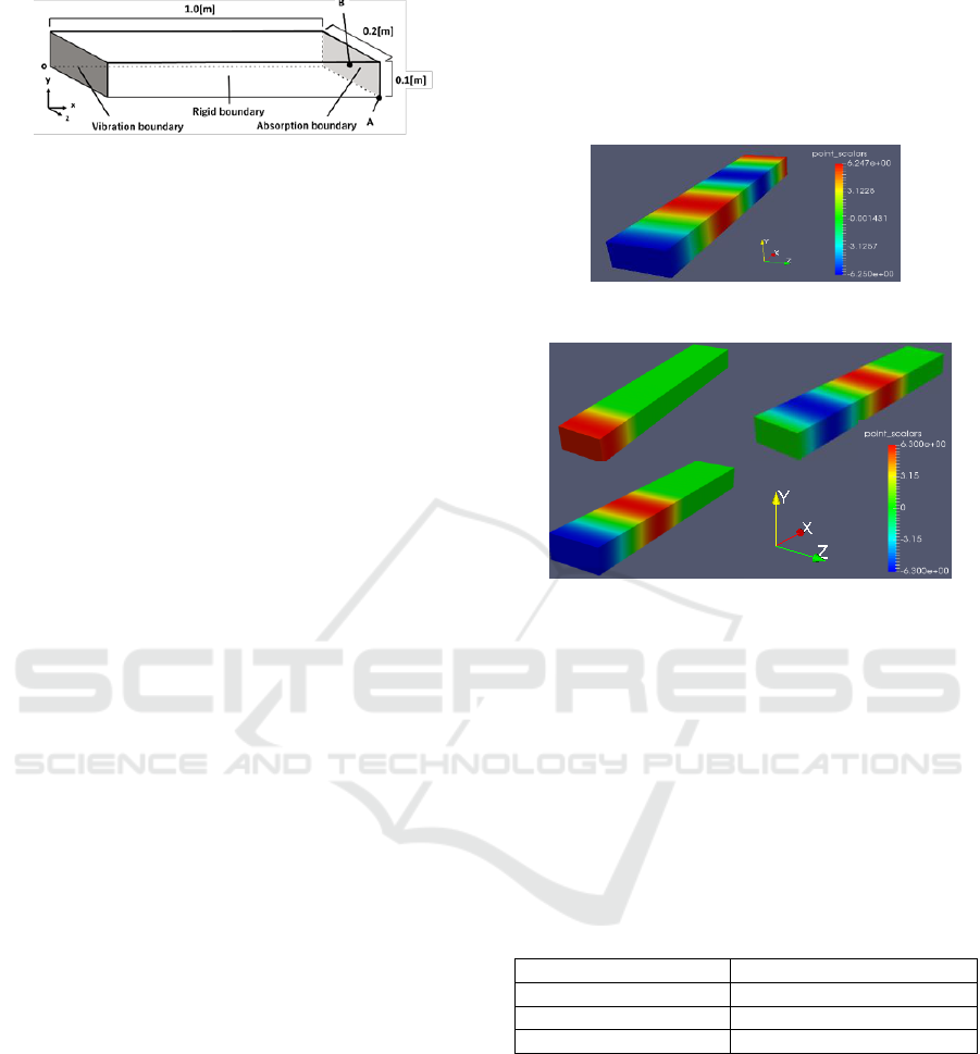
Figure 4: AHLV100.
4 PERFORMANCE EVALUATION
4.1 Benchmark Model
An acoustic problem benchmark model is used to
verify our method. The analysis uses the test model
AHLV100 of Code_Aster known as a representative
benchmark problem of acoustic problems. The model
is shown in Figure 4.
This model is an acoustic tube having a length of
1 [m], a height of 0.1 [m] and a width of 0.2 [m], and
has a vibration boundary (sound source) at the left end
and a sound absorption boundary at the right end.
Specific acoustic impedance
[kg/m
3
s]
is given as a sound absorbing boundary condition.
The analysis environment uses 1 PC equipped
with Intel Core i7-8700 multi-core CPU and 32GB of
memory.
4.2 ADVENTURE System
ADVENTURE system is a generic term for a group
of system modules in a large-scale computational
dynamics development project for design
(ADVENTURE Project, Accessed on: April 15,
2019). The system is developed by several
universities research groups. ADVENTURE project
is centered at the University of Tokyo. This system
has the following features.
(1). Analysis by meshes of hundreds to 100 million
degrees of freedom is possible.
(2). Even in a parallel computing environment of
2,000 processors, high parallel efficiency can be
achieved.
(3). It is free and open source.
(4). Scalability and maintainability are secured by
standardization of modular structure and I/O.
In this research, the ADVENTURE system is used
for analysis model creation, mesh generation, and
setting of boundary conditions.
4.3 Analysis Result (AHLV100)
The results of a steady-state analysis of AHLV100 are
shown in Figure 5, and the results of transient state
analysis are shown in Figure 6.
Figure 5: Result of steady-state.
Figure 6: Result of transient state.
From Figure 6, the acoustic phenomenon of the
closed tube can be confirmed. Also, it can be
confirmed that the plane wave from the sound source
propagates vertically in the x-direction.
Table 1 shows the results of accuracy verification.
Here, the verification is performed at the time when
the sound pressure distribution becomes the same as
the solution shown in Figure 5. Comparison with the
reference solution is made at node A belonging to the
sound absorbing surface shown in Figure 4.
Table 1: Analysis result.
Point
A
Theoretical [Pa]
6.0237
Numerical [Pa]
5.9721
Error [%]
-0.8566
4.4 Analysis of Real Environment
Model
Perform analysis based on the real environment to
confirm whether large-scale analysis is possible. The
analysis target is a small acoustic environment (live
house). This is a model based on an existing live
house. The appearance and dimensions of the analysis
target are shown in Figure 7 and Figure 8.
The live house model used has a shape that
simulates a sound source, a stage, human bodies, and
(1)
(2)
(3)
Research and Development of High Performance Finite Element for Large Scale Acoustic Analysis Method
357
structures inside. From the sound source, a sound
pressure of 0.2 [Pa] is released where assuming the
performance of the instrument is given as a tone burst.
Sound absorption boundary conditions are set to the
specific acoustic impedance, the floor is set to wood,
and other wall surfaces and structures are set to glass
wool. The cylinder that simulates the human body
gives the boundary condition as total stiffness. The
medium is air 1.2 [
], the speed of sound is
340[m/s] and the frequency is 560 [Hz].
The analysis environment is a PC cluster
composed of 25 PCs (100 cores) equipped with a
multicore CPU of Intel Core i7 2600K (3.4GHz / L2
256KB x4 / L3 8MB) and 32GB of memory.
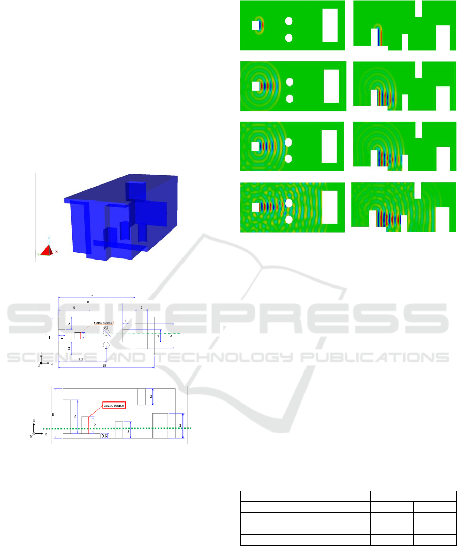
Figure 7: Appearance of model shape.
(a) Z axis viewpoint [m].
(b) Y axis viewpoint [m].
Figure 8: Dimensions of model shape.
4.5 Analysis Result (Live House)
The visualization results of the sound pressure viewed
from the Y, Z axes directions are shown in Figure 9(a)
and (b). Visualization is the result of the green dotted
line in Figure 8.
4.6 Higher Order Elements
For large-scale analysis, in addition to the
development of solvers as described above, the
reduction of the number of necessary elements is also
an issue. Therefore, in addition to the commonly used
(a) Z axis
(b) Y axis
Figure 9: Appearance of model shape.
2nd order elements, authors introduce 3rd order
elements. This is introduced to the non-parallel code
which is the test code described above. The analysis
target is AHLV100 shown in 4.1. Analysis frequency
is 1 [kHz], 2 [kHz].
The analysis results of the error rate of 0.5 [%] are
shown in Table 2. Where, NOE is number of
elements, NOI is number of iterations and NOD is
number of divisions.
From these results, it can be seen that the number
of elements is greatly reduced by the introduction of
the high-order elements, and highly accurate analysis
can be performed with a small number of divisions.
The impact is particularly large when the frequency
is high. However, further reduction of the number of
elements is necessary for practical use.
Table 2: Analysis result (high order element).
Freq.
1 [kHz]
2 [kHz]
Nth elm.
2
3
2
3
NOE
822
142
24 808
1 487
NOI
274
122
2 867
2 180
NOD
6.92
3.86
10.8
4.22
5 CONCLUSIONS
This paper describes a large-scale acoustic analysis
method using a parallel finite element method based
SIMULTECH 2019 - 9th International Conference on Simulation and Modeling Methodologies, Technologies and Applications
358

on the IDDM, and discusses the introduction of high
order elements.
In the transient analysis using the test model
AHLV100, the analysis was performed correctly, and
the usefulness of this method could be confirmed.
Also shown that transient analysis can be performed
correctly even in real environmental problems such as
the live house.
Moreover, it was shown that high precision
analysis is possible to reduce the number of elements
by introducing high order element. In particular, it
was found that the higher the frequency, the greater
the benefit of high order elements. By introducing this
into the parallelized code, further efficiency of
analysis can be expected.
However, application to large-scale and complex
sound environments requires further reduction of the
number of elements. For this reason, to introduce
high-performance elements such as the partition of
unity FEM (PUFEM) with high tracking ability to
waveforms, and promote research and development.
REFERENCES
Otsuru T., et. Al, 2002. Large Scale Sound Field Analysis
by Finite Element Method onto Rooms with
Temperature Distribution, Proc. of ICSV 9/CD-ROM.
London, 2
nd
edition.
Sendo Y., et. Al., 2002. FDTD (2, 4) method for high
precision 3D sound field analysis, Institute of
Electronics, Information and Communication
Engineers (IEICE) Academic journal A, Vol.J85-A,
No.8, pp.833-839. (In Japanese).
Sakuma T., Yasuda. Y., 2009. Sound environment
numerical simulation by high speed multipole boundary
element method, Japan Society for Simulation
Technology (JSST) Academic journal Vol. 28, No3,
pp.106-111. (In Japanese).
Okuzono K., et. Al., 2010. Fundamental accuracy of time
domain finite element method for sound-field analysis
of rooms. journal ISSN, Vol. 71, Issue 10, pp. 940-946.
Urata Y., 2004. Three-dimensional sound field analysis by
analytical solution (Simulation and experiment of free
and forced vibration). Proceeding Japan Society of
Mechanical Engineers (JSME), Vol. 70, No. 699,
pp.3091-3098. (In Japanese)
Murakami Y., Yamamoto K., Takei A., 2019. Development
and Validation of Parallel Acoustic Analysis Method
for the Sound Field Design of a Large Space.
ICBDL2018, AISC 744, pp. 206-214.
AIJ, 2011. The book, Acoustic Numerical Simulation –
Techniques and Applications of Wave Acoustic
Analysis-. AIJ. Japan, 1st edition.
Ogino M., Takei A., et. Al., 2016. A numerical study of
iterative substructuring method for finite element
analysis of high frequency electromagnetic fields.
Computers and Mathematics with Applications (2016),
DOI: 10. 1016 / j. camwa.
Takei A., Sugimoto S., Ogino M., Yoshimura S., Kanayama
H., 2010. Full Wave Analyses of Electromagnetic
Fields with an Iterative Domain Decomposition
Method. IEEE Transactions on Magnetics, Vol. 46, No.
8(2010), pp.2860-2863.
Mandel J., 1993. Balancing domain decomposition. Comm.
Numer. Methods Engrg., pp.233-241.
ADVENTURE Project Home Page: [Online]. Aveilable:
https://adventure.sys.t.u-tokyo.ac.jp/, Accessed on:
April 15, 2019.
Research and Development of High Performance Finite Element for Large Scale Acoustic Analysis Method
359
