Farm Detection based on Deep Convolutional Neural Nets

and Semi-supervised Green Texture Detection using

VIS-NIR Satellite Image

Sara Sharifzadeh

, Jagati Tata

and Bo Tan

Faculty of Engineering, Environment and Computing, Coventry University, Gulson Rd, Coventry CV1 2JH, U.K.

Faculty of Information Technology and Communication Sciences, Tampere University, Tampere, Finland

Keywords: Classification, Supervised Feature Extraction, Convolutional Neural Nets (CNNs), Satellite Image, Digital

Agriculture.

Abstract: Farm detection using low resolution satellite images is an important topic in digital agriculture. However, it

has not received enough attention compared to high-resolution images. Although high resolution images are

more efficient for detection of land cover components, the analysis of low-resolution images are yet important

due to the low-resolution repositories of the past satellite images used for timeseries analysis, free availability

and economic concerns. The current paper addresses the problem of farm detection using low resolution

satellite images. In digital agriculture, farm detection has significant role for key applications such as crop

yield monitoring. Two main categories of object detection strategies are studied and compared in this paper;

First, a two-step semi-supervised methodology is developed using traditional manual feature extraction and

modelling techniques; the developed methodology uses the Normalized Difference Moisture Index (NDMI),

Grey Level Co-occurrence Matrix (GLCM), 2-D Discrete Cosine Transform (DCT) and morphological

features and Support Vector Machine (SVM) for classifier modelling. In the second strategy, high-level

features learnt from the massive filter banks of deep Convolutional Neural Networks (CNNs) are utilised.

Transfer learning strategies are employed for pretrained Visual Geometry Group Network (VGG-16)

networks. Results show the superiority of the high-level features for classification of farm regions.

1 INTRODUCTION

Land cover classification and object-specific

classification using Earth’s observing satellites have

been some of the most important applications of

remote sensing. In digital agriculture domain, farm

detection is a key factor for different applications

such as diagnosis of diseases and welfare-

impairments, crop yield monitoring and surveillance

and control of micro-environmental conditions an

important topic in digital agriculture domain

(Stephanie Van Weyenberg, Iver Thysen, Carina

Madsen, 2010; Schmedtmann and Campagnolo,

2015; Vorobiova, 2016; Leslie, Serbina and Miller,

2017)

There have been advancements in computer

science leading to the launch of high-resolution

sensors. Yet, it remains fundamental to study and use

https://orcid.org/0000-0003-4621-2917

https://orcid.org/0000-0002-6855-6270

Low-resolution satellite imagery that is being used

since more than 30 years. The higher resolution

offered by new sensors surely overcome the

limitations related to accuracy. However, the

continuity of the existing low-resolution systems data

is crucial. A work reported in (Rembold et al., 2013),

is an example that uses low-resolution Landsat

imagery for crop monitoring and yield forecasting,

expanding their operational systems. Furthermore,

time series investigation, for example change

detection, requires comparison with low resolution

images of the old databases (Canty and Nielsen, 2006;

Tian, Cui and Reinartz, 2014). In addition, analysing

high resolution satellite images requires more

processing time and higher cost (Fisher et al., 2018).

As discussed in (Fisher et al., 2018), the achieved

accuracy can be affected by some limiting factors

such as the variations in sensor angle and increase in

100

Sharifzadeh, S., Tata, J. and Tan, B.

Farm Detection based on Deep Convolutional Neural Nets and Semi-supervised Green Texture Detection using VIS-NIR Satellite Image.

DOI: 10.5220/0007954901000108

In Proceedings of the 8th International Conference on Data Science, Technology and Applications (DATA 2019), pages 100-108

ISBN: 978-989-758-377-3

shadows. Such factors challenge the precision of

spatial rectification. Then, considering the trade-off

between accuracy and cost, and depending on the

application, the value and need for higher-resolution

data must be analysed. Therefore, low resolution

satellite images such as Landsat are appropriate for

detection of large features such as farms (Leslie,

Serbina and Miller, 2017).

Reviewing the literature shows a vast amount of

research performed in land-cover classification. Early

works utilized pixel-based unsupervised and

supervised techniques such as Neural Networks

(NN), decision trees and nearest neighbours

(HARDIN. P.J, 1994; Hansen, Dubayah and Defries,

1996; Paola and Schowengerdt, 1997). Then, sub-

pixel, knowledge-based, object-based and other

hybrid classification techniques became prevalent.

Examples can be found (Foody and Cox, 1994;

Ryherd and Woodcock, 1996; Stuckens, Coppin and

Bauer, 2000). In many of those works software and

computational tools such as ERDAS and Khoros 2.2

were extensively utilized (Stuckens, Coppin and

Bauer, 2000). Recently, eCognition and ArcGIS

softwares have been utilized widely (Juniati and

Arrofiqoh, 2017; Fisher et al., 2018); A review of

some remote sensing classification studies can be

found in (Lu and Weng, 2007), where feature

extraction and, discrimination techniques for object

classification, such as urban areas and crops are

addressed.

One of the challenges of software-based strategies

is their low accuracy when applied on low resolution

images like Landsat 8 (Juniati and Arrofiqoh, 2017).

In such cases, appropriate choice of training samples,

segmentation parameters and modelling strategy is

important; for example, suitable segmentation scale

to avoid over and under segmentation is vital for

Object Based Image Analysis OBIA. Although there

are several reports of superior performance on

different landscapes, due to the segmentation scale

issue and lower resolution, OBIA is not very ideal for

Landsat data (Juniati and Arrofiqoh, 2017).

Another group of strategies utilise saliency maps for

pixel level classification of high-resolution satellite

images mainly. Examples are spectral domain

analysis such as Fourier and wavelet transforms for

creation of local and global saliency maps (Zhang and

Yang, 2014; Zhang et al., 2016) and combined low

level SIFT descriptors, middle-level features using

locality-constrained linear coding (LLC) and high

level features using deep Boltzmann machine (DBM)

(Junwei Han, Dingwen Zhang, Gong Cheng, Lei Guo,

2015).

In addition, the state of the art CNNs have been used

recently for classification of satellite images (Albert,

Kaur and Gonzalez, 2017; Fu et al., 2017;

Muhammad et al., 2018). Due to the limited

effectiveness of manual low-level feature extraction

methods in highly varying and complex images such

as diverse range of land coverage in satellite images,

deep feature learning strategies have be applied

recently for ground coverage detection problems. One

of the effective deep learning strategies is the deep

CNNs due to its bank of convolutional filters that

enables quantification of massive high-level spectral

and spatial features.

In this paper, the problem of farm detection using

low resolution satellite images is addressed. Two

main strategies are considered and compared.

The first strategy is based on the traditional

feature extraction and SVM classification techniques,

similar example works in different domains are (Jake

Bouvrie , Tony Ezzat, 2008; Sharifzadeh, Serrano and

Carrabina, 2012; Sharifzadeh et al., 2013). The

developed algorithm consists of an unsupervised

pixel-based segmentation of vegetation area using

NDMI, followed by a two-step supervised step for

texture area classification and farm detection; at the

first step GLCM and 2-D DCT features are used in an

SVM framework for texture classification and in the

second step, object-based morphological features

were extracted from the textured areas for farm

detection.

The second strategy utilises the deep high-level

features of pre-trained CNNs. The VGGNet16 is used

and the activation vectors are utilised for farm

detection problem using transfer learning strategy.

The rest of paper is organized as follows; section

2 is about data description. Section 3 describes the

both classification strategies. The experimental

results are presented in section 4 and we finally

conclude in section 5.

2 DATA DESCRIPTION

Landsat 8 is the latest earth imaging satellite of the

Landsat Program operated by the EROS Data Centre

of United States Geological Survey (USGS), in

collaboration with NASA. The spatial resolution of

the images is 30m. Landsat 8 captures more than 700

scenes per day. The instruments Operational Land

Imager (OLI) and Thermal Infrared Sensor (TIRS) in

Landsat 8 have improved Signal to Noise Ratio

(SNR) and quantization of data is 12-bit to allow

better land cover analysis. The products downloaded

are 16-bit images (55,000 grey levels) (Leslie,

Farm Detection based on Deep Convolutional Neural Nets and Semi-supervised Green Texture Detection using VIS-NIR Satellite Image

101

Serbina and Miller, 2017) (Landsat.usgs.gov.

Landsat 8 | Landsat Missions). There are 11 bands out

of which, we use all the visible and infrared (IR)

bands. The chosen area for analysis is near Tendales,

Ecuador (See Figure 4). In this work, different

combinations of band are used for calculating

vegetation and moisture indices used in estimation of

vegetation green areas as well as visible RGB bands

for classification analysis.

3 METHODOLOGY

In this section the two main used classification

methodologies are explained.

3.1 Feature Extraction-based Strategy

In this strategy, the vegetation area is segmented

using the Normalized Difference Moisture Index

(NDMI) image. Next, local patches are generated

automatically, from the segmented green area. Then,

textured areas including farms or any other pattern are

classified by applying SVM on the extracted features

using GLCM and 2-D DCT. Finally, the farm areas

are detected by morphological analysis of the textured

patches and SVM modelling. MATLAB 2018 was

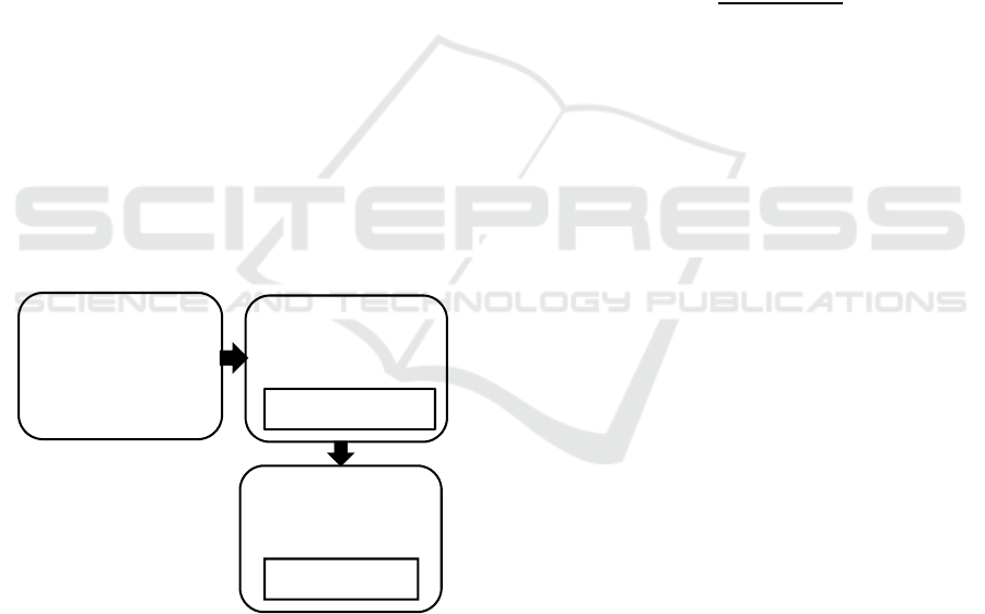
used for all implementations. Figure 1 shows the

block diagram of the analysis strategy.

Figure 1: Block diagram showing the overall process of the

first strategy.

3.1.1 Vegetation Segmentation

The pixels are segmented using spectral bands; the

Near Infra-Red (NIR) in 851-879 nm range and

Shortwave NIR (SWIR) in 1566-1651 nm range are

used. One of the common methods for vegetation

estimation is the Normalized Difference Vegetation

Index (NDVI) (Ali, 2009). However, NDMI (Ji et al.,

2011) can be a more suitable technique because it

considers the moisture content of the soil and plants

instead of the leaf chlorophyll content or leaf area.

There are also similar works like (Li et al., 2016),

which have used NDMI and tasselled cap

transformations on 30m resolution Landsat images

for estimating soil moisture. Hence, the farm areas

that went undetected by NDVI are well detected by

thresholded NDMI strategy.

NDMI uses two near-infrared bands (one channel of

1.24-µm that was never used previously for

vegetation indices) to identify the soil moisture

content. It is employed in forestry and agriculture

applications (Gao, 1996). This index has been used in

this paper for the estimation of total vegetation

including the agricultural lands and farms. For Lands

imagery, NDMI is calculated as:

NDMI 

NIRSWIR

NIRSWIR

(1)

NDMI is always in the range [-1, +1]. It is reported

that NDMI values more than 0.10- 0.20 indicate very

wet or moist soil surfaces (Ji et al., 2011). Then, based

on this study, cultivable land is extracted for further

classification.

3.1.2 Texture Area Detection

The detected green areas from the previous step are

mapped on the RGB band images. Farm areas are part

of the green areas of the image; therefore, the detected

green areas are divided into small patches of 200

200 pixels. Then, feature extraction is performed for

each patch of image to detect the textured patches.

Patches with flat patterns do not include a farm area.

GLCM - One of the feature extraction techniques

employed for texture areas is the GLCM that is

widely used for texture analysis (Tuceryan, 1992).

The GLCM studies the spatial correlation of the pixel

grayscale and spatial relationship between the pixels

separated by some distance in the image. It looks for

regional consistency considering the extent and

direction of grey level variation. Considering the

characteristics of the flat regions and the textured

regions (non-farm or farm) as shown in Figure 5,

GLCM is used for discrimination. Mathematically,

the spatial relation of pixels in image matrix is

quantified by computing how often different

combinations of grey levels co-occur in the image or

a section of the image. For example, how often a pixel

with intensity or tone value  occurs either

horizontally, vertically, or diagonally to another pixel

at distance  with the value  (see Figure 2-a).

Depending on the range of intensities in an image, a

GLCM-DCT- SVM

Green area

segmentation

(NDMI-Un sup.)

Step 1.

Tex. Vs. Flat

Feature Ext.

Step 2.

Tex. Vs. Farm

Feature Ext.

Morph. - SVM

DATA 2019 - 8th International Conference on Data Science, Technology and Applications

102

number of scales are defined and a GLCM square

matrix of the same dimensional size is formed. Then,

image pixels are quantized based on the discrete

scales and the GLCM matrix is filled for each

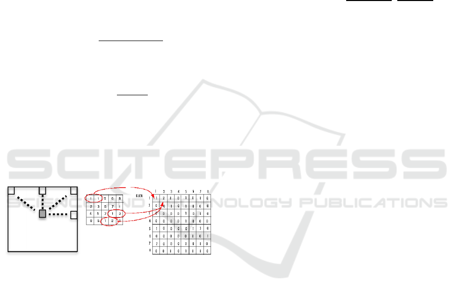
direction. Figure 2-b shows the formation process of

a GLCM matrix based on horizontal occurrences at

1. The grayscales are between 1 to maximums 8

in this case.

Two order statistical parameters: Contrast,

Correlation, Energy and Homogeneity samples are

used to define texture features in the vegetation.

Considering a grey co-occurrence matrix  , they are

defined as:

Contras



ij



pi,j

,

(2)

Correlation  

i



j



pi,j





,

(3)

Energ

pi,j



,

(4)

Homogenit



pi,j

1

ij

,

(5)

where, ,denote row and column number,



, 







,



are the means and standard deviations of 



and





, so that, 











∑

,





and 











∑

,





.  is the number of intensity scales, used

for GLCM matrix formation.

(a) (b)

Figure 2: (a) Illustration of forming GLCM matrices in four

directions i.e., 0

,45

,90

,135

. (b) Computation of

GLCM matrix based on horizontal occurrences at 1 for

an image (MATLAB, 2019).

Further detailed information can be found in

(Haralick, Dinstein and Shanmugam, 1973). The

GLCM features are calculated in directions 0°, 45°,

90°, and 135° as shown in Figure 2-a. The calculated

GLCM features in the four directions are averaged for

each parameter and used as input to the classification

model

GLCM 



Cont



,Corr



,Eng



,Hom





, (see

Table 1).

2D DCT - DCT sorts the spatial frequency of an

image in ascending order and in the form of cosine

coefficients. Most significant coefficients lie in the

lower order, corresponding to the main components

of the image, while the higher order coefficients

correspond to high variation in images. Since the

variation in a textured patch is higher than a flat one,

the DCT map can help to distinguish them. For this

aim, the original image patch 



is transformed into

DCT domain 



and a hard threshold is applied to

the DCT coefficients to remove the high order

coefficients 



. Then, the inverse 2D-DCT of

the thresholded image 



is computed. In both

original and DCT domain, the reduction in the

entropy of the textured patches is more significant

than the flat areas representing smooth variations.

Therefore, the ratio of coefficients’ entropy before

and after thresholding 

























 are

calculated in both domains. For textured patches the

entropy ratios are greater compared to flat patches

due to the significant drop in entropy after

thresholding the large amount of high frequency

information (See Figure 6).

3.1.3 Morphological Features

To recognize if a detected textured patch contains

farm areas, first the patch image is converted to

grayscale image. Then, the Sobel edge detection

followed by morphological opening and closing by

reconstruction are performed. This highlights the

farm areas, keeping the boundaries and shapes in the

image undisturbed. Next, the regional maxima were

found to extract only the areas of maximum intensity

(or the highlighted foreground regions). Further, the

small stray blobs, disconnected or isolated pixels, and

pixels having low contrast with the background in

their neighbourhood are discarded. This is because

there is a contrast between the farm regions (marked

as foreground) and their surrounding boundary pixels.

The same procedure is performed for a non-farm

sample. The area of the foreground as well as the

entropy for a patch including farm is higher compared

to a non-farm due to the higher number of connected

foreground pixels. Figure 7 shows the resulting

images of this analysis.

3.1.4 SVM Modelling

SVM classifiers are trained using the four GLCM and

the two DCT features at step 1 and morphological

features at step 2. The first model is capable to detect

textured versus the flat patches and the second one

detects the patches including farms from the textured

patches with no farm areas. The LibSVM (Chang and

Lin, 2011) is used. In this paper, the 5-fold cross-

validation (Hastie, Tibshirani and Friedman, 2009), is

used to find the optimum kernel and the

corresponding parameters. It helps to avoid over-

Pixel of interest

Farm Detection based on Deep Convolutional Neural Nets and Semi-supervised Green Texture Detection using VIS-NIR Satellite Image

103

fitting or under-fitting. The choice of kernel based on

cross validation allows classifying data sets with both

linear and non-linear behaviour. SVM was used for

remote-sensing and hyperspectral image data analysis

previously (Petropoulos, Kalaitzidis and Prasad

Vadrevu, 2012).

3.2 Transfer Learning Strategy for

VGGNet16

CNN is a popular classification method based on deep

learning different levels of both spectral and special

features using the stack of filter banks at several

convolutional layers. However, training a CNN

requires large data sets and heavy time-consuming

computations and is prone to over-fitting using small

data sets. A versatile approach in this case is transfer

learning; The high-level deep features learnt over

several layers of convolution, pooling and RELU

using million images of massive ranges of scenes and

objects are kept. That is based on the fact that the

weighted combination of these activation maps of

high-level features are the underlying building blocks

of different objects of the scenes. While, the end

layers called fully connected layers (FC) should be re-

trained using hundreds of new training images. These

layers are used to evaluate the strong correlation of

the previous layers high-level features to particular

classes of the task (in training images) and calculate

the appropriate weights giving high probabilities for

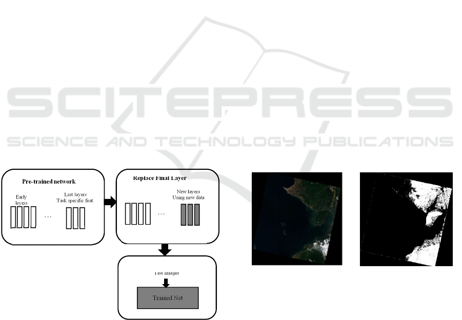
correct classifications. Figure 3 shows the transfer

learning concept.

Figure 3: Block diagram showing the transfer learning

strategy.

The recent works on utilisation of this technique

(Chaib

et al., 2017; Li et al., 2017) shows suitability

of transference of the learnt activation vectors for a

new image classification task. Therefore, new patches

of satellite images are used to retrain the final FC

layers of VGG-16 CNN.

3.2.1 VGG-16

VGG-16 network is trained on more than a million

images from the ImageNet database (Image Net,

2016). There are 16 deep layers and 1000 different

classes of objects, e.g. keyboard, mouse, pencil, and

many animals. This network has learned rich high-

level feature representing wide ranges of objects. The

size of input image is 2242243 where the three

colour layers are RGB bands. The last three FC layers

are trained for classification of 1000 classes. As

explained, these three layers are retrained using our

satellite image patches of the same size for farm

classification while all other layers are kept.

4 EXPERIMENTAL RESULTS

In this section the results obtained from both

strategies are presented and compared.

4.1 Feature Extraction Strategy

Results

As mentioned in section 2, the Landsat 8 satellite

images source is used. Figure 4-a shows the image

used in this work.

(a) (b)

Figure 4: (a) Landsat 8 RGB image of Tendales, Ecuador

(b) Result of thresholding using the NDMI.

Figure 4-b shows the result of vegetation green

area detection using NDMI. This image was further

utilised for making patches (from green areas) that are

used for the two-step classification framework.

Figure 5 shows three patches of flat, textured-farm

and textured non-farm areas.

New layers

Using new data

Replace Final Layer

…

Fewer classes (10s),

less data (100s)

Early

layers

Last layers

Task specific feat.

Pre-trained network

…

1000s classes,

Millions of images

Test Images

New trained net

Trained Net

roved Net

DATA 2019 - 8th International Conference on Data Science, Technology and Applications

104

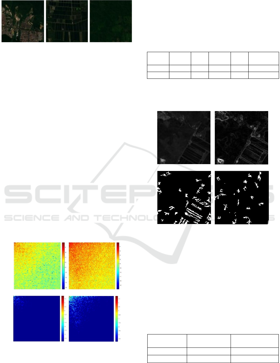
(a) (b) (c)

Figure 5: Examples of (a) Flat (b) Textured-Farm (c)

Textured Non-Farm patches.

In the experiments of both steps of feature

extraction and classification with SVM, the number

of training patches of both classes (textured verses

flat and farm verses non- farm) were almost balanced

to avoid discriminative hyperplanes found by SVM

be favoured toward the more populated class. Totally

from total patches, around 75% was used for training

and the rest were kept as unseen data for test. In the

first classification, 111 samples were used for training

and 15 samples for test. In the second classification,

there were 83 training samples and 22 test samples.

At the first step, the four GLCM features and two

DCT features were extracted from patches and

combined. Figure 6 visualises the 2D DCT maps of a

flat and textured patch before thresholding the higher

frequencies coefficients and after thresholding. As

can be seen, the textured patch has high energies in

both low frequencies as well as high frequencies,

while in the flat patch DCT map, only low

coefficients show high energy values. Therefore, the

thresholded DCT map of the textured patch shows

significant drop of energies in high frequencies. This

influences the entropy ratios.

(a) (b)

Figure 6: DCT map before thresholding (a) flat patch, (b)

textured patch. After thresholding (c) flat patch (d) textured

patch.

Table 1 presents the average of the GLCM and

DCT features over 20 patches for textured and flat

classes.

Table 1: GLCM and one of the DCT features used for

classification of Flat and Textured Areas. (Values shown

are averaged over 20 samples).

Class Cont. Eng. Hom. Ent.

DCT Ent.

Ratio

Flat

0.0041 0.991 0.9979 3.014 0.1202

Tex.

0.067 0.847 0.9671 4.761 0.3337

All the classified textured patches from this step

were used to extract the morphology features at the

second step, as shown in Figure 7.

(a) (b)

Figure 7: (a) Grayscale image of a farm patch (b) Result of

Sobel edge detection (c) Detected farm area by

morphological foreground detection (d) Detected area of a

textured non-farm patch shown in Figure 5-a.

The performance of classifiers is evaluated based

on the number of correctly classified samples. Results

are presented in Table 2. As can be seen, the first

texture classification step is very robust. However,

the performance is reduced for the second farm

classifier based on morphology features.

Table 2: Training and test accuracy of the two-step feature

extraction-based strategy for farm detection.

Classification

Step

Train Accuracy

(%)

Test Accuracy (%)

1 96.39 (107/111) 93.33 (14/15)

2 83.1325 (69/83) 81.8182 (18/22)

Farm Detection based on Deep Convolutional Neural Nets and Semi-supervised Green Texture Detection using VIS-NIR Satellite Image

105

4.2 Transfer Learning Strategy Results

In order to retrain the three FC layers of VGG-16 net,

hundreds of images are required. Then, further

number of patches were used compared to the first

strategy to fulfil the requirements of this modelling

strategy. Transfer learning was performed using three

different sets of more than 300 patches. The first set

includes image patches from any general area of the

satellite image, including ocean patches, mountains,

residential areas, green flat and textured areas and

farms. The last three FC layers of VGG-16 were

retrained for the two-class farm detection problem.

In the second set, the same number of patches

were used excluding the non-green areas based on

NDMI. This means the patches can include one of the

flat green area, green textured non-farm area or a farm

area.

Finally, in the third set of the same size, only

green textured non-farm patches as well as farm ones

were used.

In all three cases, 75% of patches were used for

training and the remaining was used as the test unseen

data. There were 72 farm patches and the rest were

non-farm in all three sets. Due to random selection,

the number of patches of each class are different in

the generated sets. The average and standard

deviation of the results over 5 randomly generated

train and test sets are reported in Table 3. As

expected, no significant difference can be seen

between the results of the three studies. That is, the

high-level features acquired from the stack of filter

banks include all those spectral, special, structural

and colour features extracted using the manual feature

extraction strategy. Due to inclusive level of features

extracted using the deep convolutional layers, the

CNN results outperform the two-step feature

extraction strategy.

Table 3: Average and standard deviation of the training and

test accuracy of the CNN using transfer learning on the

three different sets of patches.

Classification

type

Train Accuracy (%) Test Accuracy (%)

Farm vs. general

areas

99.550.64 96.762.26

Farm vs. green

areas 

99.370.76 95.952.87

Farm vs. green

tex. area

98.910.52 96.76 2.80

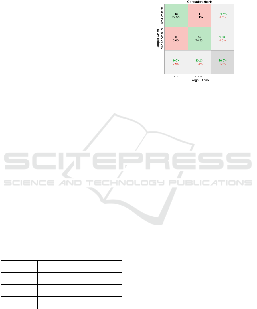
Figure 8, shows the confusion matrix of one of the

five test sets results using the transferred CNN

models. The first experiment data set, that classifies

farm patches from any general patch was used. As

shown, only one general non-farm patch was

misclassified as a farm patch.

Figure 8: The confusion matrix of one of the five test sets

results from the first data set (classification of farm patches

from any general patch).

5 CONCLUSIONS

This paper is focused on farm detection using low

resolution satellite images. Two main detection

strategies are considered; first a traditional feature

extraction and modelling strategy was developed. In

this method, unsupervised thresholding using

Normalized Difference Vegetation Index (NDVI)

was used for green area detection. Then, a two-step

algorithm was developed using Grey Level Co-

occurrence Matrix (GLCM), 2D Discrete Cosine

Transform (DCT) and morphological features as well

as Support Vector Machine (SVM) modelling to

detect the farms areas from textured areas. The

second strategy was based on deep high-level features

learnt from the pre-trained Visual Geometry Group

Network (VGG-16) networks. In order to use these

features for farm classification, transfer learning

strategies were employed. The experimental results

showed the superiority of the Convolutional Neural

Networks (CNN) models.

REFERENCES

Albert, A., Kaur, J. and Gonzalez, M. (2017) ‘Using

convolutional networks and satellite imagery to identify

patterns in urban environments at a large scale’.

Available at: http://arxiv.org/abs/1704.02965.

Ali, A. (2009) Comparison of Strengths and Weaknesses of

NDVI and Landscape-Ecological Mapping Techniques

for Developing an Integrated Land Use Mapping

Approach A case study of the Mekong delta , Vietnam

Comparison of Strengths and Weaknesses of NDVI and

DATA 2019 - 8th International Conference on Data Science, Technology and Applications

106

Landscape-Ecolo, ITC. International Institute for Geo-

Information Science and Earth Observation.

Canty, M. J. and Nielsen, A. A. (2006) ‘Visualization and

unsupervised classification of changes in multispectral

satellite imagery’, International Journal of Remote

Sensing, 27(18), pp. 3961–3975.

Chaib, S. et al. (2017) ‘Deep Feature Fusion for VHR

Remote Sensing Scene Classification’, IEEE

Transactions on Geoscience and Remote Sensing.

IEEE, 55(8), pp. 4775–4784.

Chang, C. and Lin, C. (2011) ‘LIBSVM : A Library for

Support Vector Machines’, ACM Transactions on

Intelligent Systems and Technology (TIST), 2, pp. 1–39.

Fisher, J. R. B. et al. (2018) ‘Impact of satellite imagery

spatial resolution on land use classification accuracy

and modelled water quality’, Remote Sensing in

Ecology and Conservation, 4(2), pp. 137–149.

Foody, G. M. and Cox, D. P. (1994) ‘Sub-pixel land cover

composition estimation using a linear mixture model

and fuzzy membership functions’, International

Journal of Remote Sensing.

Fu, G. et al. (2017) ‘Classification for high resolution

remote sensing imagery using a fully convolutional

network’, Remote Sensing, 9(5), pp. 1–21. doi:

10.3390/rs9050498.

Gao, B. (1996) ‘NDWI—A normalized difference water

index for remote sensing of vegetation liquid water

from space’, Remote Sensing of Environment,

266(April), pp. 257–266.

Hansen, M., Dubayah, R. and Defries, R. (1996)

‘Classification trees: An alternative to traditional land

cover classifiers’, International Journal of Remote

Sensing.

Haralick, R. M., Dinstein, I. and Shanmugam, K. (1973)

‘Textural Features for Image Classification’, IEEE

Transactions on Systems, Man and Cybernetics.

Hardin. P. J (1994) ‘Parametric and nearest-neighbor

methods for hybrid classification’, a comparison of pixel

assignment accuracy. Photogramtnetric Engineering and

Remote Sensing. 60, 60(12), pp. 1439–1448.

Hastie, T., Tibshirani, R. and Friedman, J. (2009) The

elements of statistical learning. Second Edi. New York:

Springer.

Image Net (2016) Stanford Vision Lab, Stanford University,

Princeton University. Available at: http://www.image-

net.org/ (Accessed: 12 January 2019).

Jake Bouvrie , Tony Ezzat, and T. P. (2008) ‘Proceedings

of International Conference On Acoustics, Speech and

Signal Processing’, in Localized Spectro-Temporal

Cepstral Analysis of Speech, pp. 4733–4736.

Ji, L. et al. (2011) ‘On the terminology of the spectral

vegetation index (NIR-SWIR)/(NIR+SWIR)’, Interna-

tional Journal of Remote Sensing, 32(21), pp. 6901–

6909.

Juniati, E. and Arrofiqoh, E. N. (2017) ‘Comparison of

pixel-based and object-based classification using

parameters and non-parameters approach for the pattern

consistency of multi scale landcover’, in ISPRS

Archives. International Society for Photogrammetry

and Remote Sensing

, pp. 765–771.

Junwei Han, Dingwen Zhang, Gong Cheng, Lei Guo, and J.

R. (2015) ‘Object Detection in Optical Remote Sensing

Images Based on Weakly Supervised Learning and

High-Level Feature Learning’, IEEE Transactions on

Geoscience and Remote Sensing, 53(6), pp. 3325–3337.

Landsat.usgs.gov. Landsat 8 | Landsat Missions (no date)

https://earthexplorer.usgs.gov/. Available at:

https://landsat.usgs.gov (Accessed: 17 May 2018).

Leslie, C. R., Serbina, L. O. and Miller, H. M. (2017)

‘Landsat and Agriculture — Case Studies on the Uses

and Benefits of Landsat Imagery in Agricultural

Monitoring and Production: U.S. Geological Survey

Open-File Report’, p. 27.

Li, B. et al. (2016) ‘Estimating soil moisture with Landsat

data and its application in extracting the spatial

distribution of winter flooded paddies’, Remote

Sensing, 8(1).

Li, E. et al. (2017) ‘Integrating Multilayer Features of

Convolutional Neural Networks for Remote Sensing

Scene Classification’, IEEE Transactions on

Geoscience and Remote Sensing.

Lu, D. and Weng, Q. (2007) ‘A survey of image

classification methods and techniques for improving

classification performance’, International Journal of

Remote Sensing.

MATLAB (2019) Graycomatrix, R2019a.

Muhammad, U. et al. (2018) ‘Pre-trained VGGNet

Architecture for Remote-Sensing Image Scene

Classification’, Proceedings - International Conference

on Pattern Recognition. IEEE, 2018–Augus (August),

pp. 1622–1627.

Paola, J. D. and Schowengerdt, R. a (1997) ‘The Effect of

Neural-Network Structure on a Classification’,

Americal Society for Photogrammetry and Remote

Sensing, 63(5), pp. 535–544.

Petropoulos, G. P., Kalaitzidis, C. and Prasad Vadrevu, K.

(2012) ‘Support vector machines and object-based

classification for obtaining land-use/cover cartography

from Hyperion hyperspectral imagery’, Computers and

Geosciences. Elsevier, 41, pp. 99–107.

Rembold, F. et al. (2013) ‘Using low resolution satellite

imagery for yield prediction and yield anomaly

detection’, Remote Sensing, 5(4), pp. 1704–1733. doi:

10.3390/rs5041704.

Ryherd, S. and Woodcock, C. (1996) ‘Combining Spectral

and Texture Data in the Segmentation of Remotely

Sensed Images’, Photogrammetric engineering and

remote sensing.

Schmedtmann, J. and Campagnolo, M. L. (2015) ‘Reliable

crop identification with satellite imagery in the context

of Common Agriculture Policy subsidy control’,

Remote Sensing.

Sharifzadeh, S. et al. (2013) ‘DCT-based characterization

of milk products using diffuse reflectance images’, in

2013 18th International Conference on Digital Signal

Processing, DSP 2013.

Sharifzadeh, S., Serrano, J. and Carrabina, J. (2012)

‘Spectro-temporal analysis of speech for Spanish

phoneme recognition’, in 2012 19th International

Farm Detection based on Deep Convolutional Neural Nets and Semi-supervised Green Texture Detection using VIS-NIR Satellite Image

107

Conference on Systems, Signals and Image Processing,

IWSSIP 2012.

Stephanie Van Weyenberg, Iver Thysen, Carina Madsen, J.

V. (2010) ICT-AGRI Country Report, ICT-AGRI

Country Report. Reports on the organisation of research

programmes and research institutes in 15 European

countries. Available at: http://ict-agri.eu/sites/ict-

agri.eu/files/deliverables/ICT-Agri-country_report.pdf.

Stuckens, J., Coppin, P. R. and Bauer, M. E. (2000)

‘Integrating contextual information with per-pixel

classification for improved land cover classification’,

Remote Sensing of Environment.

Tian, J., Cui, S. and Reinartz, P. (2014) ‘Building change

detection based on satellite stereo imagery and digital

surface models’, IEEE Transactions on Geoscience and

Remote Sensing, 52(1), pp. 406–417.

Tuceryan, M. (1992) ‘Moment based texture

segmentation’, in Proceedings - International

Conference on Pattern Recognition. Institute of

Electrical and Electronics Engineers Inc., pp. 45–48.

Vorobiova, N. S. (2016) ‘Crops identification by using

satellite images and algorithm for calculating estimates’,

in CEUR Workshop Proceedings, pp. 419–427.

Zhang, L. et al. (2016) ‘Global and local saliency analysis

for the extraction of residential areas in high-spatial-

resolution remote sensing image’, IEEE Transactions

on Geoscience and Remote Sensing. IEEE, 54(7), pp.

3750–3763.

Zhang, L. and Yang, K. (2014) ‘Region-of-interest

extraction based on frequency domain analysis and

salient region detection for remote sensing image’,

IEEE Geoscience and Remote Sensing Letters, 11(5),

pp. 916–920.

DATA 2019 - 8th International Conference on Data Science, Technology and Applications

108