Software Modularity Coupling Resolution by the Laplacian of a

Bipartite Dependency Graph

Iaakov Exman and Netanel Ohayon

Software Engineering Dept., The Jerusalem College of Engineering – JCE-Azrieli, Jerusalem, Israel

Keywords: Modularity, Dependency Graph, Bipartite Dependency Graph, Laplacian Matrix, Eigenvectors, Coupling

Types, Coupling Resolution, Bipartition Idea.

Abstract: Software modularity by pinpointing and subsequent resolution of the remaining coupling problems is often

assumed to be a general approach to optimize any software system design. However, software coupling

types with differing specific characteristics, seemingly pose serious impediments to any generic coupling

resolution approach. Despite the diversity of types, this work proposes a generic approach to solve any

coupling type in three steps: a- obtain the Dependency graph for the coupled modules; b- convert the

dependency graph into a Bipartite Graph; c- generate the Laplacian Matrix from the Bipartite Graph.

Coupling problems to be resolved are then located, using Laplacian eigenvectors, in particular the Fiedler

eigenvector. The generic approach is justified, explained in detail, and illustrated by a few case studies.

1 INTRODUCTION

On the way to formulate a generic, linear algebraic

theory of software composition, it was natural to

start from basic notions of object-oriented design,

such as classes and their methods. The columns and

rows of matrices, representing hierarchical levels of

software systems, stand for generalizations of

classes and their methods (Exman, 2013), as shown

in sub-section 1.1 on the Laplacian matrix (Exman

and Sakhnini, 2016, 2018).

But, one would expect a more comprehensive

theory of software systems composition to treat,

besides classes and methods, additional concepts

considered coupling causes.

The existence of different coupling types –

concisely reviewed in Sub-section 1.2 – responsible

for a variety of obstacles to software system design,

led researchers to assume that a generic solution to

software coupling would be difficult to achieve.

The generic resolution of coupling problems is

the goal of this paper, as stated in sub-section 1.3.

Indeed, it is attainable by the combination of a

dependency graph displaying couplings of any type,

with the computational techniques offered by the

Laplacian matrix, itself generated from graphs,

obtaining the desired generic coupling resolution

approach.

1.1 Laplacian Matrix Concepts

Software systems are assumed to be hierarchical,

with the lowest level composed of classes and their

methods. Going upwards, with increasing

abstraction, classes are clustered into modules, in

turn further clustered into bigger modules, sub-

systems and finally the whole software system.

There are a few ways to formally represent an

abstraction level. This paper focuses on two kinds of

display: a bipartite graph and a Laplacian Matrix.

A bipartite graph (Weisstein, 2019a) contains

two sets of entities; each entity, shown as a graph

vertex, is linked by edges only to entities in the other

set. Typical entities are a set of structors denoted by

, a generalization of classes for any level, and a set

of functionals denoted by F

, a generalization of

class methods. Edges link classes to the methods

they provide. An abstract bipartite graph in Fig. 1,

shows modules, their structors and functionals.

A Laplacian Matrix L (Weisstein, 2019b) is

generated from a graph according to equation (1):

LDA





(1)

where D is the Degree Matrix showing the degree

Deg(v

) of vertex v

in its diagonal element D

A is

the Adjacency Matrix, with A

= 1 for each i, j

vertex pair in the graph, and A

= 0 otherwise.

298

Exman, I. and Ohayon, N.

Software Modularity Coupling Resolution by the Laplacian of a Bipartite Dependency Graph.

DOI: 10.5220/0007955802980305

In Proceedings of the 14th International Conference on Software Technologies (ICSOFT 2019), pages 298-305

ISBN: 978-989-758-379-7

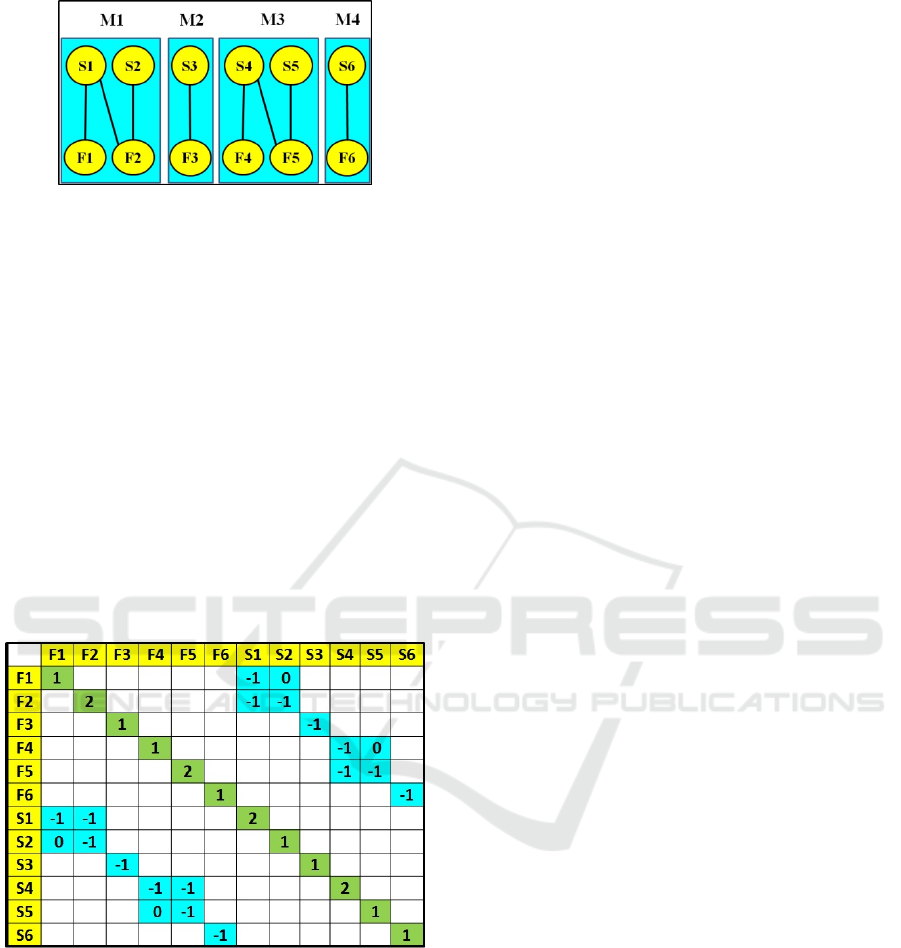
Figure 1: Schematic bipartite graph of a software system –

it shows 6 structors (S1 to S6), 6 functionals (F1 to F6)

and 4 modules (M1 to M4), separated by the underlying

(blue) rectangles. (Color online).

The Laplacian Matrix (Fig. 2) is generated from

the bipartite graph (Fig.1). Properties of interest are:

 The Laplacian matrix is symmetric;

 The number of modules in a Laplacian – i.e. the

graph connected components – is the number of

zero-valued Laplacian eigenvalues.

 The Fiedler vector (Fiedler, 1973) (de Abreu,

2007) fits the 1

positive Laplacian eigenvalue;

its vector element signs (positive/negative)

enable splitting a module into smaller modules.

Note that modules may contain smaller “modules”.

To avoid confusion we may denote smaller ones by

vertices, reserving the modules term for larger ones.

Figure 2: Schematic Laplacian Matrix generated from the

bipartite graph in Fig. 1 – It has a diagonal Degree matrix

(green background) and an Adjacency matrix (blue

background) with minus signs by eq. (1). All matrix

elements outside modules are zero-valued. (color online).

1.2 Software Coupling Types

Any list of coupling types is forcefully partial, due

to diverse views of different authors, techniques and

classification criteria – e.g. (Coupling-Wiki, 2019).

The coupling types listed in this sub-section is a

sample of the diversity, rather than a comprehensive

list. It includes, among others:

 Common Coupling – several modules access the

same global data;

 Content Coupling – one module uses the code of

other module; see below the similar CBO;

 Control Coupling – one module controls the

flow of another, by passing a what-to-do-flag;

 Coupling Between Objects (CBO) – methods of

one class call methods or access variables of

another class;

 Data Coupling – modules share data through

parameters;

 External Coupling – two modules share an

externally imposed data format;

 Stamp Coupling – modules share a composite

data structure and use only parts of it;

1.3 Goal of this Paper

This paper goal is to propose a generic approach to

coupling resolution, independent of specific

coupling types. It assumes the following premises:

 Dependency Graph – any coupling type can be

represented by a dependency graph;

 Bipartite Graph – any dependency graph can be

converted into a generic bipartite graph;

 Laplacian Analysis – one can analyse a bipartite

graph by its Laplacian matrix;

 Coupling Resolution – combines data from the

dependency and its bipartite graph.

1.4 Paper Organization

The remaining of this paper is organized as follows.

Section 2 mentions related work. Section 3 presents

the approach by means of an introductory running

example. Section 4 states preliminary theoretical

considerations and the generic procedure to coupling

resolution. Section 5 analyses case-studies. Section 6

is a discussion concluding the paper.

2 RELATED WORK

2.1 Coupling Type Classifications

An elementary coupling type classification is found

in (Coupling-Wiki, 2019). The literature up to now

informally defined coupling. For instance, in the

GoF Design Patterns book (Gamma et al., 1995)

glossary: “coupling is the degree to which software

Software Modularity Coupling Resolution by the Laplacian of a Bipartite Dependency Graph

299

components depend on each other”. It justifies our

use of the linear algebra notion of “linear

dependence” to formalize coupling.

Still, most works on this topic are empirical. An

example is (Beck and Diehl, 2011) stating that

software systems are modularized to make their

complexity manageable; but, as guiding principles

were not known, they look at different kinds of

coupling in their study. Another example of an

empirical study is by (Bavota et al., 2013).

2.2 Graph Techniques

The Program Dependence Graph (PDG) is reviewed

by (Ferrante et al., 1987). PDG is an intermediate

program representation exposing both data and

control dependencies of operations in a program. In

principle, this could be a starting point to a generic

resolution of dependencies.

A precise Bipartite Graph definition is found in

(Weisstein, 2019a). Bipartite Graphs have appeared in

many contexts. Obtaining bipartite graphs from other

graphs is relevant to this work. (Huffner, 2009) finds

the minimum vertex set to be deleted to get a bipartite

graph. From another viewpoint, (Guillaume and

Latapy, 2004) claim that any complex networks can

be viewed as bipartite structures.

2.3 Laplacian Matrix Techniques

Laplacian Matrix spectral techniques have been used

in various fields, including software engineering. A

survey on Laplacian graphs is (Merris, 1994).

A spectral clustering tutorial in (von Luxburg,

2007), stresses the Laplacian. Another review on

spectral clustering for software engineering,

especially the Laplacian, is found in (Shtern and

Tzerpos, 2012).

Ng et al., (2001) deal with spectral clustering,

analysing an algorithm, explicitly referring to the

Laplacian. Shokoufandeh et al., (2005) extract a

Module Dependency Graph (MDG) from software

source code for clustering into MDG partitions.

Their Modularization Quality criterion is

reformulated as a Laplacian eigenvalue problem.

3 A RUNNING EXAMPLE

A small Chatroom software system exemplifies our

generic approach, illustrating "coupling between

objects". The chatroom concept is from the web and

was implemented by this paper's authors in C#.

3.1 Dependency Graphs

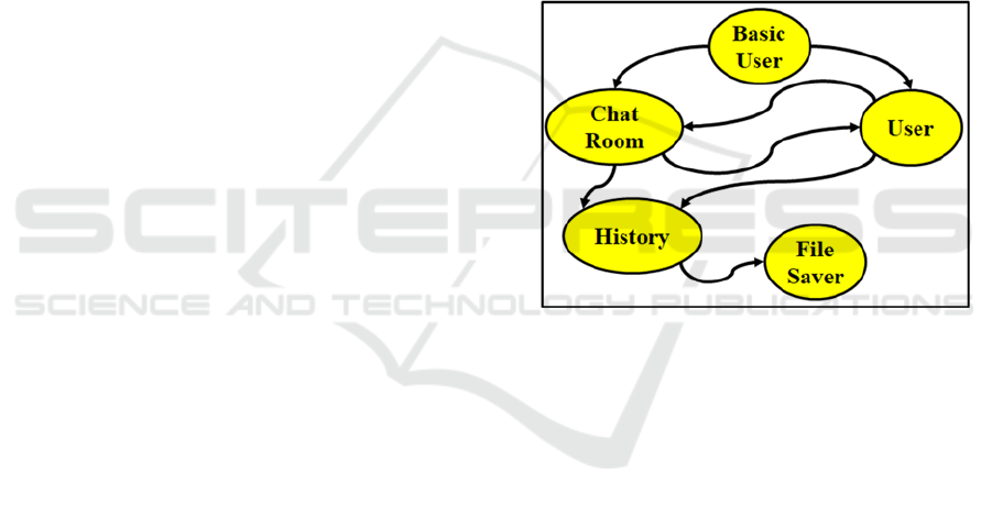
Initially one describes a system of any coupling type

by a dependency graph. We consider two cases:

 Mutual Module Dependency – in this case (e.g.

content, control, CBO and data coupling) an

arrow points from the dependent vertex to the

independent vertex;

 Two or More Modules Dependent on a 3

Party

Entity – here (e.g. common, external and stamp

coupling) arrows point from dependent modules

to the 3

party entity.

In either case one obtains a dependency graph – a

directed graph with arrows showing dependencies

between graph vertices. All coupling types are

reduced to the same generic kind of dependency

graph. Fig. 3 shows the Chatroom dependency.

Figure 3: Chatroom Dependency Graph – Arrows point

from each dependent vertex to independent vertices: e.g. the

“History” vertex is dependent on “File-Saver”.

3.2 Bipartite Graphs

In order to obtain a unique bipartite graph, from a

dependency graph, one does the following actions:

 Duplicate Each Dependency Graph Vertex into a

Vertex Pair – keep each original vertex and

another copy, prefixing with a "d" (dependent) the

original vertex name;

 Obtain Two Sets of Vertices of the Same Size –

one independent, another dependent;

 Copy Each Dependency Graph Arrow to the

Bipartite Graph – each arrow points from a

dependent vertex to an independent one.

Fig. 4 illustrates the Chatroom bipartite graph

corresponding to the dependency graph in Fig. 3.

ICSOFT 2019 - 14th International Conference on Software Technologies

300

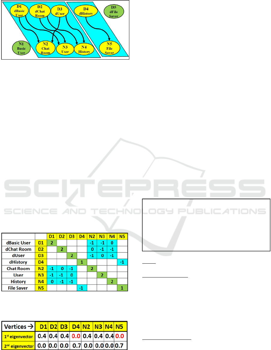
Figure 4: Chatroom Bipartite Graph – Arrows point from a

"D" dependent vertex to an "N" non-dependent vertex.

The bipartite graph itself already separates vertices into

two "modules" (blue background). Isolated vertices (N1-

BasicUser and D5-dFileSaver) are not connected at all to

other vertices. (color online).

3.3 Laplacian Matrix, Its Eigenvalues

and Eigenvectors

A software system Laplacian Matrix is generated

from its Bipartite Graph as follows:

 Choose All Vertices with at Least one

Connection Arrow - to the other bipartite graph

vertex set; ignore isolated vertices;

 Count Connection Arrows Per Vertex – to

obtain the Degree matrix;

 List Neighbours of Each Vertex – to obtain the

Adjacency matrix;

 Generate the Laplacian – inserting Degree and

Adjacency matrix values in eq. (1).

The Chatroom Laplacian Matrix in Fig. 5 was

generated from the Bipartite Graph in Fig. 4.

Figure 5: Chatroom Laplacian Matrix – Matrix generated

from the Bipartite Graph in Fig. 4. All matrix elements

outside modules are zero-valued. (color online).

Figure 6: Chatroom Laplacian Eigenvectors – Two

eigenvectors fit the two zero-valued eigenvalues. Each

eigenvector shows one of the connected components; for

instance, the 2nd eigenvector vertices are (D4, N5).

The number of zero-valued eigenvalues of this

matrix gives the number of its connected

components. Calculation obtains 2 such eigenvalues.

The respective eigenvectors are seen in Fig 6.

The Fig. 6 eigenvectors show the connected

components – the Chatroom modules – neatly

corresponding to the Fig. 4 modules. A more

detailed case study analysis is done in section 5.

4 THEORETICAL

CONSIDERATIONS AND

GENERIC PROCEDURE

4.1 Modules Bipartition

The first generic procedure step to deal with module

coupling obtains a dependency graph. This is a

necessary information collection step, telling which

modules are dependent on other ones.

This work central innovative idea is the

transition from a dependency to a bipartite graph.

Bipartition contributes to modules decoupling,

which is somewhat surprising since no new specific

software system information is added in the

transition from the dependency to its bipartite graph.

The next lemma states bipartition uniqueness.

Proof:

The proof is by construction.

Forward Direction – Duplicate all the dependency

graph vertices, into a list of vertex pairs. Prefix the

name of the 1

element of each vertex pair by the

letter "d" (for dependent). One obtains two vertex

sets – a dependent and a non-dependent set – of

equal size. Scan top-down and left-to-right, copying

each dependency graph arrow to a single arrow

linking a dependent to a non-dependent vertex. The

result is the unique bipartite graph.

Backward Direction – Take only the bipartite graph

set of non-dependent vertices. Copy this set to a

fresh vertex set in a blank area.

Scan left-to-right, the bipartite graph arrows; copy

each bipartite graph arrow to the respective elements

Lemma 1: Unique directed Bipartite Graph

from Coupling Dependency Graph

The bipartite graph, linking a set of vertices

standing for dependent modules to another set of

vertices standing for non-dependent modules,

generated from a given Coupling Dependency

Graph, is unique.

Software Modularity Coupling Resolution by the Laplacian of a Bipartite Dependency Graph

301

of the fresh vertex set. The result restores the initial

forward direction dependency graph.

Now we state some convenient definitions about

possible components of the bipartite graph. These

definitions are better understood, when illustrated by

the vertices of Fig. 4.

4.2 Laplacian Matrix for Modules

Decoupling

Having a directed bipartite graph fitting the modules

dependency graph of a software system, one

generates the bipartite graph Laplacian matrix and

calculates the system modules number and sizes.

Proof:

The straightforward proof is again by construction.

From the directed bipartite graph:

a. Generate the Adjacency Matrix;

b. Generate the Degree Matrix D;

c. Generate the Laplacian by equation (1) of

section 1.1, viz.



 .

This construction is illustrated e.g. in Fig. 5.

It is straightforward to obtain the number of the

software system modules and their sizes from the

Laplacian Matrix. This is given by the next theorem.

Proof:

Decoupling modules are connected components of

the directed bipartite graph generated in turn from

the respective dependency graph. The Laplacian is

obtained from this bipartite graph. This theorem

directly follows from the Laplacian matrices spectral

theorem, see e.g. (von Luxburg, 2007) page 4,

proposition 2. The number of a graph connected

components is the number of its Laplacian zero-

valued eigenvalues. Component sizes are obtained

from the respective eigenvectors.

Some specific cases of decoupling modules

recognized by the relevant Laplacian Matrix are

mentioned in Lemma 3.

Proof:

These decoupled modules are recognized as

connected components

4.3 Generic Coupling Resolution

Procedure

Our generic coupling resolution procedure consists

in a series of steps, which were presented and

illustrated in previous sections.

The main steps consisting of:

 generation of the bipartite graph from the

dependency graph;

Definitions 1: Bipartite Graph Components

Convergence Point – this is a non-dependent

vertex to which at least two arrows point;

Divergence Point – this is a dependent vertex

from which at least two arrows point to two non-

dependent vertices;

Simple arrow – this is a single arrow linking one

dependent vertex to one non-dependent vertex;

Isolated dependent vertex - it is a named "d"

vertex that actually has no arrow linking to a

non-dependent vertex;

Isolated non-dependent vertex - it is a vertex that

actuall

has no arrow from a de

endent vertex;

Theorem 1: Software System decoupling

Modules’ Number and Sizes from the

Laplacian Matrix

The number and sizes of the decoupling modules

of a software system at a given abstraction level

is obtained from the Laplacian Matrix of the

directed bipartite graph generated from its

dependency graph as follows:

The module number is the number of zero-

valued Laplacian eigenvalues;

The module sizes are given by the respective

indicator eigenvectors of the zero-valued

Laplacian ei

envalues.

Lemma 3: Specific decouplin

module cases

from the Laplacian Matrix – Specific cases

recognized as individual decoupling modules

are:

a) Simple arrows;

b) Single convergence/divergence point

modules;

c) Composite modules with overlapping

conver

ence/diver

ence

oints;

Lemma 2: Unique Laplacian Matrix from the

Directed Bipartite Graph – a unique Laplacian

is generated from the directed Bipartite Graph of

a given software system, while ignoring isolated

vertices.

ICSOFT 2019 - 14th International Conference on Software Technologies

302

 generation of the Laplacian Matrix from the

bipartite graph;

are formal, very precise and represent the novel

contribution of this work.

On the other hand:

 the generation of the dependency graph;

 the information combination from both

dependency and bipartite graphs for coupling

resolution;

 the final coupling resolution by modification of

the software system;

are informal, and demand reasonable judgment

based on the software engineer experience.

Here we finally provide the whole procedure in a

pseudo-code format, in the next box.

The necessity of combining information of the

dependency and the bipartite graphs is illustrated as

follows. Suppose there are two mutually crossing

"simple arrows", viz. from vertex DA to B and from

vertex DB to A. This is the bipartite information, i.e.

apparently two independent modules. But, by the

information given by the dependency graph this is

an obvious problematic cycle that must be resolved.

5 CASE STUDY ANALYSIS

We analyse two case studies. The first is our running

example, the Chatroom. The second is an improved

Chatroom with an added Mediator design pattern.

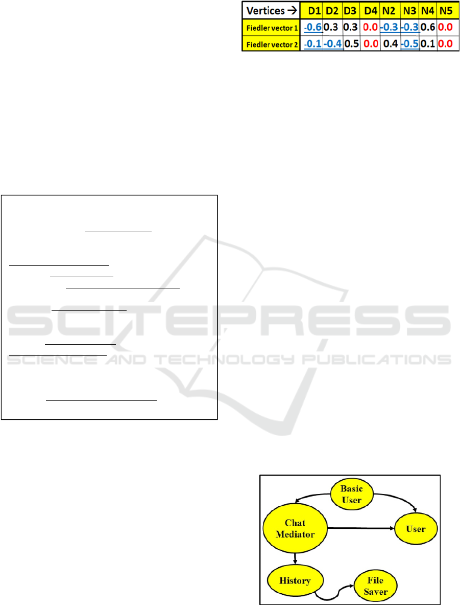
Figure 7: Chatroom Laplacian Fiedler Eigenvectors –

These eigenvectors enable further splitting of the big

composite module. The Fiedler vector 1 has minus signs

marking vertices (D1, N2, N3). The Fiedler vector 2 marks

vertices (D1, D2, N3). (color online).

5.1 The Chatroom Software System

The modules obtained for Chatroom running

example, by the Laplacian Matrix eigenvectors (in

Fig. 6), correspond to a "simple arrow" – containing

the vertices

(D4, N5)

– and a "composite module"

with overlapping convergence/divergence points –

containing all the remaining vertices, except the

isolated ones. These comply with Lemma 3.

Additional calculation of Fiedler eigenvectors for

the Chatroom system, obtains the results in Fig. 7.

Note that further splitting by Fiedler vectors

obtains a single divergence point module (D1, N2,

N3) and a single convergence point module (D1, D2,

N3); it again complies with Lemma 3, i.e. modules

are recognized by their relatively dense connections.

5.2 Improved Chatroom with a

Mediator Pattern

An obvious decoupling of the Chatroom "composite

module", in Fig. 4, uses a Mediator Pattern. The

natural Mediator candidate is the Chatroom "vertex"

itself, the medium to exchange User messages.

This simple system has a single Mediator; by the

GoF book (Gamma et al., 1995) a concrete mediator

is enough (no abstract class needed). From the

arrows linked to the User, just one starting from the

ChatMediator is left in Fig. 8. It has a clearer design.

Figure 8: ChatMediator Dependency graph – simplified

dependencies decouple the big "composite" module of the

original Chatroom (in Fig. 3). (Color online).

Generic Couplin

Resolution Procedure

Obtain the coupling dependency graph of the software

system;

Translate the coupling dependency graph into a

bipartite dependency graph;

Obtain the Laplacian Matrix from the bipartite graph;

Calculate the eigenvalues and eigenvectors of the

Laplacian Matrix;

Obtain the decoupling modules of the bipartite graph

from the previous eigenvalues and eigenvectors;

If judged necessary: split the decoupling modules

using the Fiedler eigenvector of the Laplacian matrix;

Locate module couplings to be resolved, based on

joint information from the dependency and bipartite

graphs;

Modify the software system design after deciding

about the coupling resolution procedure, e.g. adding a

suitable design pattern.

Software Modularity Coupling Resolution by the Laplacian of a Bipartite Dependency Graph

303

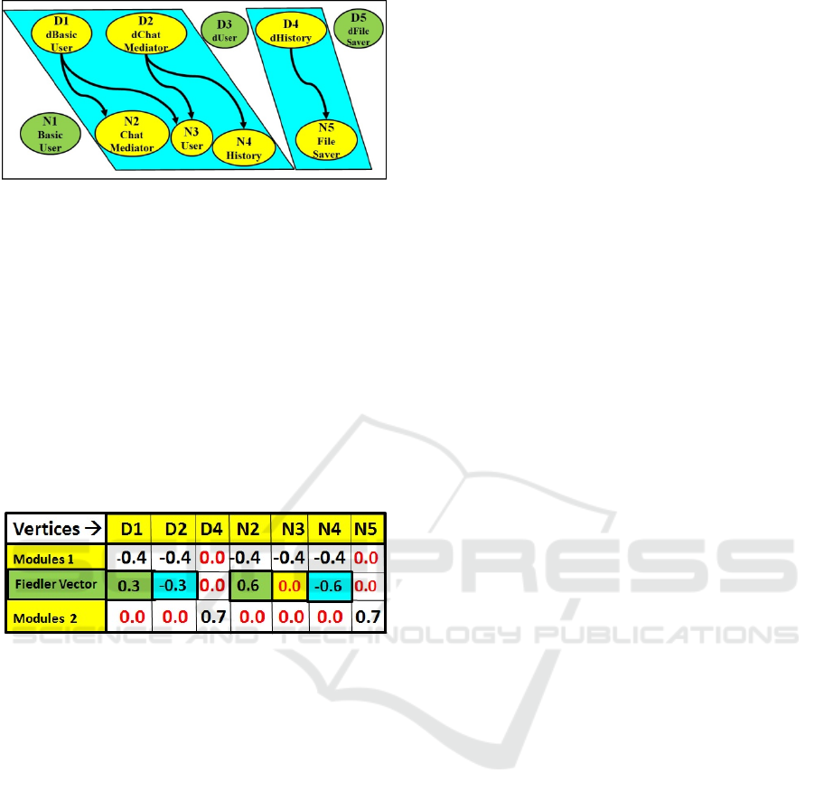
Figure 9: ChatMediator Bipartite Graph – with the same

conventions as in Fig. 4. Vertex D3 is disconnected from

the composite left-hand-side module (in Fig. 4), resulting

into “two single-divergence points”. (Color online).

Fitting the ChatMediator Dependency graph in

Fig. 8, is the Bipartite graph shown in Fig. 9.

Calculating the Laplacian Matrix eigenvectors (Fig.

10) obtains modules (marked in Fig. 9). The Fiedler

vector further splits Modules-1 by disconnecting the

N3 User vertex. This is consistent with the D3 dUser

disconnected vertex. Again, it is seen that least

connected vertices are candidates for further

disconnection, leaving modules that are recognized

by their relatively dense connections.

Figure 10: ChatMediator Eigenvectors – Modules-1 fits

the left-hand-side module in Fig. 9. Modules-2 fits the

right-hand-side module in Fig. 9. The Fiedler vector

enables further splitting of Modules-1, by disconnecting

vertex N3, leaving two smaller modules: (D1, N2) and

(D2, N4), according to the Fiedler vector elements’ sign.

6 DISCUSSION

6.1 The Bipartition Idea

Bipartition is the central innovative idea of this

work, as already stated in Sub-section 4.1.

Bipartition is obtained by taking an "arrow" of

the dependency graph and bisecting it into a source

and a destination – i.e. the dependent and the non-

dependent entities. This apparently trivial act

increases our understanding, enabling easier

decoupling.

Bipartition can be compared to an intriguing idea

in quantum computation – see e.g. (Kong et al.,

2018) and (Makaruk, 2017) – in which instead of

moving a particle from one state to another, one uses

an annihilation operator in the source state and a

creation operator in the destination state. In other

words, one decomposes a "transfer" between states

into two parts, the disappearance from the source

state and reappearance in the destination state.

6.2 Linear Dependence in Linear

Algebra

Why is the Laplacian Matrix so smart to recognize

correctly the modules that should be decoupled? The

answer relies in the concept of linear dependence in

linear algebra, as a satisfactory representation of

"dependence" in software systems.

6.3 Further Case Studies

As part of this research work, we have tested the

generic approach to any coupling types, in particular

the use of Bipartition, on additional small and

medium size case studies, on systems found in the

internet, and developed by software engineers, other

than the authors of this paper,

As an example of such a case study, we have

applied the approach to “Stateless”, an open source

project (Stateless, 2019), containing a .Net library to

create state machines in C#. The results obtained

with the additional case studies are similar to those

in this paper. These additional results, which due to

space limitations cannot be included here, are

planned to appear in an extended version of this

work.

6.4 Future Work

This paper presented novel ideas. Work should be

done to exploit these ideas using an extensive and

representative sample of larger software systems, to

test their applicability and scalability.

6.5 Main Contributions

The two main contributions of this work are: 1- to

approach all types of coupling in a uniform manner;

2- to introduce bipartition as a generic way to apply

linear algebra to decouple modules in a variety of

situations.

REFERENCES

Bavota, G., Dit, B., Oliveto, R., Di Penta, M.,

Poshyvanyk, D. and De Lucia, A., 2013. “An

ICSOFT 2019 - 14th International Conference on Software Technologies

304

Empirical Study on the Developers’ Perception of

Software Coupling”, Proc. ICSE’2013 Int. Conf. on

Softw. Eng., San Francisco, IEEE Press, pp. 692-701.

Beck, F. and Diehl, S., 2011. “On the Congruence of

Modularity and Code Coupling”, in Proc. 19

Sigsoft

Symposium ESEC/FSE’11, Szeged, Hungary, pp. 354-

364. DOI: 10.1145/2025113.2025162

Cai, Y. and Sullivan, K.J., 2006. “Modularity Analysis of

Logical Design Models”, in Proc. 21

IEEE/ACM Int.

Conf. Automated Software Eng. ASE’06, pp. 91-102,

Tokyo, Japan.

Coupling_(computer_programming)-Wikipedia, 2019.

https://en.wikipedia.org/wiki/Coupling

de Abreu, N.M.M., 2007. “Old and new results on

algebraic connectivity of graphs”, Linear Algebra and

its Applications, 423, pp. 53-73. DOI:

https://doi.org/10.1016/j.laa.2006.08.017

Exman, I., 2012. “Linear Software Models”, Extended

Abstract, in I. Jacobson, M. Goedicke and P. Johnson

(eds.), SEMAT Workshop on GTSE, pp. 23-24, KTH,

Stockholm, Sweden. Video: http://www.youtube.com/

watch?v=EJfzArH8-ls

Exman, I., 2013. “Linear Software Models are Theoretical

Standards of Modularity”, in J. Cordeiro, S.

Hammoudi, and M. van Sinderen (eds.): ICSOFT

2012, Revised selected papers, CCIS, Vol. 411, pp.

203–217, Springer-Verlag, Berlin, Germany. DOI:

10.1007/978-3-642-45404-2_14

Exman, I., 2014. “Linear Software Models: Standard

Modularity Highlights Residual Coupling”, Int.

Journal on Software Engineering and Knowledge

Engineering, vol. 24, pp. 183-210, March 2014. DOI:

10.1142/S0218194014500089

Exman, I., 2015. “Linear Software Models: Decoupled

Modules from Modularity Eigenvectors”, Int. Journal

on Software Engineering and Knowledge Engineering,

vol. 25, pp. 1395-1426, October 2015. DOI:

10.1142/S0218194015500308

Exman, I. and Sakhnini, R., 2016. “Linear Software

Models: Modularity Analysis by the Laplacian

Matrix”, in Proc. 11

ICSOFT Int. Joint Conference

on Software Technologies, Lisbon, Portugal, Vol. 2:

ICSOFT-PT, pages 100-108. DOI:

10.5220/0005985601000108.

Exman, I. and Sakhnini, R., 2018. “Linear Software

Models: Bipartite Isomorphism between Laplacian

Eigenvectors and Modularity Matrix Eigenvectors”,

Int. Journal of Software Engineering and Knowledge

Engineering, Vol. 28, No. 7, pp. 897-935. DOI:

10.1142/S0218194018400107

Ferrante, J., Ottenstein, K.J. and Warren, J.D., 1987. “The

Program Dependence Graph and Its Use in

Optimization”, ACM Trans. Prog. Lang and Systems,

Vol. 8, pp. 319-349.

Fiedler, M., 1973. “Algebraic Connectivity of Graphs”,

Czech. Math. J., Vol. 23, (2) 298-305 (1973).

Gamma, E., Helm, R., Johnson, R. and Vlissides, J., 1995.

Design Patterns: Elements of Reusable Object-

Oriented Software, Addison-Wesley, Boston, MA.

Guillaume, J-L. and Latapy, M., 2004. “Bipartite Structure

of all complex networks”. Inf. Proc. Let. Vol. 90, pp.

215-221/

Huffner, F., 2009. “Algorithm Engineering for Optimal

Graph Bipartization”, J. Graph Algorithms and

Applications, vol. 13, pp. 77-98.

Kong, X., Wei, S., Wen, J. and Long, G-L, 2018.

“Experimental Simulation of Bosonic Creation and

Annihilation Operators in a Quantum Processor”,

arXiv:1809.03352.

Makaruk, H.E., 2017. “Quantum computing and second

quantization”, Journal of Knot Theory and its

Ramifications, Vol. 26, 1741006. DOI:

https://doi.org/10.1142/S0218216517410061

Merris, R., 1994. "Laplacian matrices of graphs: a survey",

Linear Algebra and its Applications, Vols. 197-198,

January-February, pp. 143-176. DOI: 10.1016/0024-

3795(94)90486-3.

Ng, A.Y., Jordan, M.I., and Weiss, Y., 2001. “On spectral

clustering: analysis and an algorithm”, in: Proc. 2001

Neural Information Processing Systems, pp.849–856.

Shokoufandeh, A., Mancoridis, S., Denton, T. and

Maycock, M., 2005. “Spectral and meta-heuristic

algorithms for software clustering,” Journal of

Systems and Software, vol. 77, no. 3, pp. 213–223.

Shtern, M. and Tzerpos, V., 2012. “Clustering

Methodologies for Software Engineering”, in

Advances in Software Engineering, vol. 2012, Article

ID 792024 (2012). DOI: 10.1155/2012/792024

Stateless – a .Net library to create state machines, 2019,

https://github.com/dotnet-state-machine/stateless

von Luxburg, U., 2007. “A Tutorial on Spectral

Clustering”, Statistics and Computing, 17 (4), pp. 395-

416. DOI: 10.1007/s11222-007-9033-z

Weisstein, E.W., 2019a. “Bipartite Graph”, Wolfram.

http://mathworld.wolfram.com/BipartiteGraph.html

Weisstein, E.W., 2019b. “Laplacian Matrix”, Wolfram

http://mathworld.wolfram.com/LaplacianMatrix.html.

Software Modularity Coupling Resolution by the Laplacian of a Bipartite Dependency Graph

305