
IFOSMONDI: A Generic Co-simulation Approach Combining Iterative
Methods for Coupling Constraints and Polynomial Interpolation for
Interfaces Smoothness
Yohan
´
Eguillon
1 a
, Bruno Lacabanne
2
and Damien Tromeur-Dervout
1 b
1
Institut Camille Jordan, Universit
´
e de Lyon ,UMR5208 CNRS-U.Lyon1, Villeurbanne, France
2
Siemens Industry Software, Roanne, France
Keywords:
Solver Coupling, Iterative Co-simulation, Rollback, Polynomial Interpolation, Fixed-point Method.
Abstract:
This paper introduces IFOSMONDI co-simulation algorithm that combines iterative coupling methods and
a smooth representation of interface variables. In explicit (i.e. non-iterative) coupling methods, representing
smooth interface variables requires the introduction of a delay (Busch, 2016) because the values of the interface
variables at the end of a given macro-step are not known when the co-simulation only reached the beginning
of this very macro-step. One of the advantages of implicit co-simulation (i.e. iterative coupling methods) is
that the values of the interface variables can be known at the end of a macro-step with the possibility to replay
the integration on this very macro-step. Combining this with a polynomial representation of the interface
variables enables to use interpolation instead of extrapolation across the macro-steps (K
¨
ubler and Schiehlen,
2000). Taking into account time-derivatives of interface variables makes it possible to ensure C
1
smoothness
even with no history of the past exchanged data: then, no delay is introduced. A new possibility then arises:
the solvers of each subsystem may take into account this smoothness and be less restrictive on their restarts
due to the communication times. The results obtained on the test case of the two mass oscillators (Busch,
2016) show the advantage of IFOSMONDI coupling in terms of trade-off between elapsed time and accuracy.
1 INTRODUCTION
Industrial applications of simulations have reached a
point where modular models are not only convenient
but mandatory. Indeed, model providers are often
specialized in a precise range of physical fields such
as thermodynamic, mechanic, fluids or electrical cir-
cuits. One of the consequences of this is the necessity
of dealing with modular systems built by connecting
several subsystems where each of them embeds a part
of the physics of the global model. In the case where
the subsystems also embed a solver (which may differ
between different subsystems), the simulation of the
global system can be run by simulating each subsys-
tem separately with regular communications of data
between subsystems. This is co-simulation.
The co-simulation method (or co-simulation al-
gorithm) is the rule which deals with this meta-
simulation level by defining the times of the data com-
munications, the inputs that each subsystem should
a
https://orcid.org/0000-0002-9386-4646
b
https://orcid.org/0000-0002-0118-8100
use at each step, the way the outputs are used and
so on. Many co-simulation algorithms have been
established until now (K
¨
ubler and Schiehlen, 2000)
(Arnold and Unther, 2001) (Gu and Asada, 2004)
(Bartel et al., 2013) (Sicklinger et al., 2014) (Li et al.,
2014) (Busch, 2016) (Schweizer et al., 2016), with
various complexity of implementation, subsystems
capabilities requirements, or physical field-specific
principles (see also the recent state of art on co-
simulation of (Gomes et al., 2018)). It may appear
in some co-simulation algorithms that a time interval
should be integrated more than once on one or more
subsystems. This is called iterative co-simulation.
The systems that need to do so must have the capabil-
ity to replay a simulation over this time-interval with
different data (time to reach, input values, ...). De-
pending on the model provider, this capability called
”rollback” is not always available on every subsys-
tem. Besides the rollback, other plateform-dependent
capabilities may lead to an impossibility of use of a
given co-simulation method on certain subsystems.
Amongst them, the ability to provide inputs with n
th
176
Éguillon, Y., Lacabanne, B. and Tromeur-Dervout, D.
IFOSMONDI: A Generic Co-simulation Approach Combining Iterative Methods for Coupling Constraints and Polynomial Interpolation for Interfaces Smoothness.
DOI: 10.5220/0007977701760186
In Proceedings of the 9th International Conference on Simulation and Modeling Methodologies, Technologies and Applications (SIMULTECH 2019), pages 176-186
ISBN: 978-989-758-381-0
Copyright
c
2019 by SCITEPRESS – Science and Technology Publications, Lda. All rights reserved
order time-derivatives and the ability to obtain the
time-derivatives of the outputs at the end of a macro-
step can be mentioned.
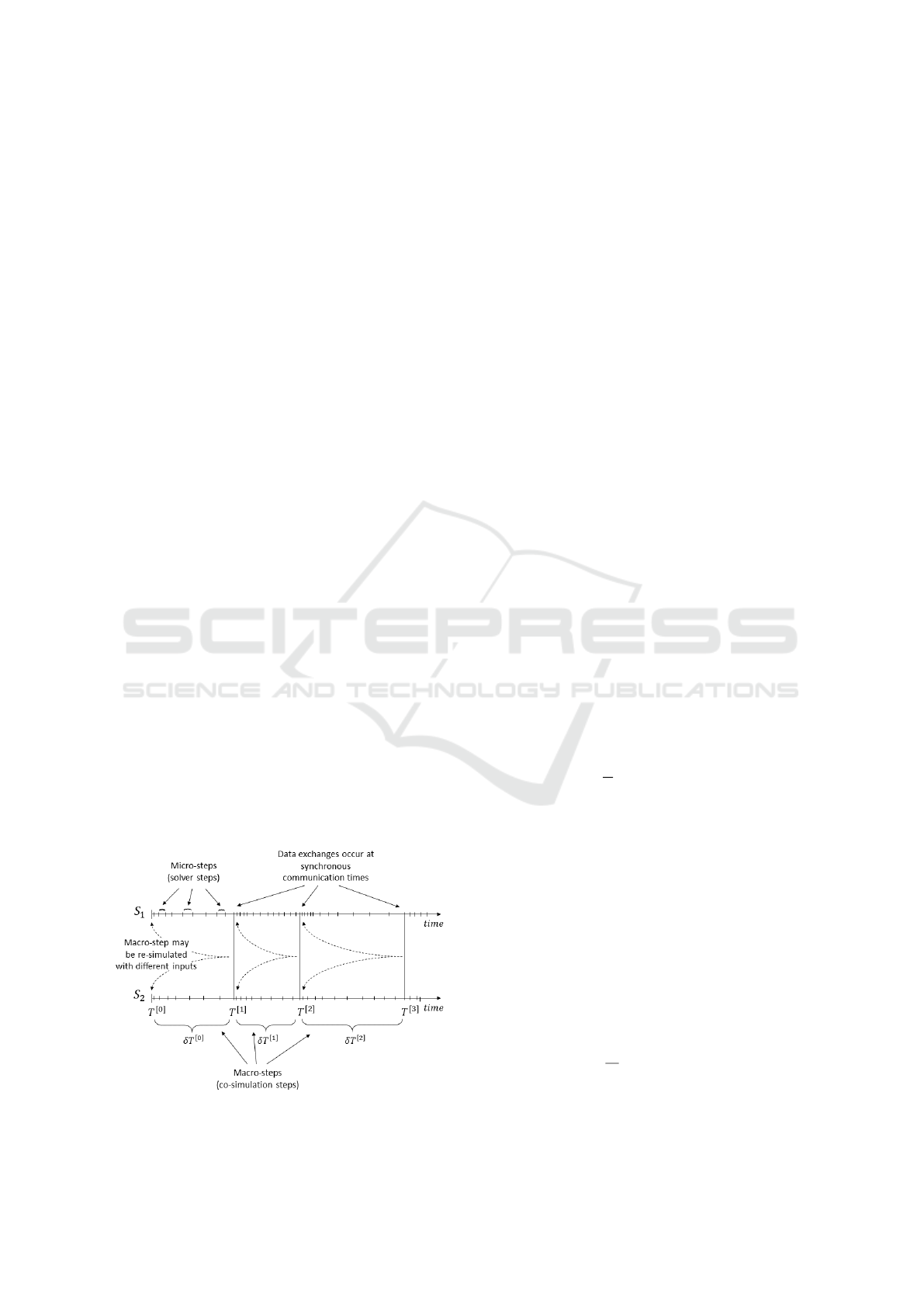
In this paper we present a synchronous and it-
erative co-simulation algorithm called IFOSMONDI
coupling as presented on figure 1 where the dynami-
cal sub-systems are solved iteratively on a macro-step
before exchanging data between sub-systems to start
the solving on a new macro-step. We propose a stan-
dardisation on the multiple principles present in co-
simulation algorithms so that fields-specificities van-
ish and that it could hence be applied on any model.
The two salient features needed by our algorithm are
the rollback capability and the ability to obtain the
time-derivatives of the outputs.
This algorithm is inspired by two main meth-
ods previously developped in (K
¨
ubler and Schiehlen,
2000) and (Busch, 2016).(K
¨
ubler and Schiehlen,
2000) introduces the modular description of dynamic
systems on the mathematical model description level.
They presented an iterative method based on quasi-
Newton on the system of nonlinear algebraic equa-
tions on the outputs, after having proceeded to the
elimination of the inputs between subsystems. Their
simulator coupling with iteration on the global inte-
gration step uses interpolation for the inputs in the
integration procedure based on the history of inputs
at past macro-steps and the updated inputs given by
the quasi-Newton. In (Busch, 2016), an approxima-
tion method denoted as extrapolated interpolation is
proposed in order to circumvent the discontinuity is-
sue of the input at the end of each macro-step but
only in the context of Gauss-Seidel and parallel Ja-
cobi schemes (Skelboe, 1992) (non iterative proce-
dure within a macro step). This paper proposes an al-
gorithm that takes advantage of these two approaches
which, once combined, allow us to have a more nu-
merically efficient method than each independently.
Figure 1: Visualization of the behavior of a synchronous
and iterative co-simulation method on 2 subsystems.
The plan of the paper is as follows. Section 2
presents the mathematical formalism we used to de-
velop the co-simulation algorithm which is consti-
tuted of subsystems framework, link function giv-
ing the data connectivities between subsystems and
coupling constraint. Then section 3 gives the IFOS-
MONDI coupling algorithm showing how the com-
bining of the iterative method and the continuity con-
straints interact. The macro step-size selection is also
given. Section 4 gives the results of IFOSMONDI
coupling on the classical linear two-mass oscillator
test case (see (Schweizer et al., 2016) for example)
where the parameters spring and damping constants
are chosen to have more stiff dynamics. Compari-
son of IFOSMONDI coupling with the algorithm of
(K
¨
ubler and Schiehlen, 2000) and the algorithm of
(Busch, 2016) is also achieved. Section 5 gives the
conclusion.
2 MATHEMATICAL
FORMALISM AND
MOTIVATIONS
A subsystem that communicates with other subsys-
tems to form a co-simulation configuration will be
represented by its equation. As the context is about
time integration, these equations will be time differ-
ential equations. First of all, we present the general
form of a monolithic system, in other words a closed
system (which neither has inputs nor outputs) repre-
sented by a 1
st
order differential equation which cov-
ers, among others things, ODE, DAE and IDE as fol-
lows:
F(
d
dt
x, x,t) = 0
x(t
init
) = x
[0]
(1)
where
n
st
∈ N
∗
, x
[0]
∈ R
n
st
, t ∈ [t
init
,t
end
],
[t
init
,t
end
] ⊂ R so that t
end
−t
init
∈ R
∗
+
,
F : R
n
st
× R
n
st
× [t
init
,t
end
] → R
n
st
,
(2)
are given, and
x : [t
init
,t
end
] → R
n
st
(3)
is the solution state vector with its n
st
components
called the state variables.
This paper will only cover the ODEs case, which
are of the form (4). The terms ”equation”, ”equa-
tions”, and ”differential equations” will refer to the
ODE of a system in the whole document.
d
dt
x = f (t,x) (4)
where
f : [t
init
,t
end
] × R
n
st
→ R
n
st
(5)
IFOSMONDI: A Generic Co-simulation Approach Combining Iterative Methods for Coupling Constraints and Polynomial Interpolation for
Interfaces Smoothness
177

2.1 Subsystems Framework
In a cosimulation context, the principle to link the
derivatives of the states to them (and potentially the
time) is the same as in the monolithic case, yet the
inputs and outputs have to be considered.
Let n
sys
∈ N
∗
be the number of subsystems. Please
note that the case n
sys
= 1 corresponds to a monolithic
system. The cases that will be considered here are
connected subsystems, that is to say n
sys
> 2 subsys-
tems that need to exchange data to one another: each
input of each subsystem has to be fed by an output of
another subsystem. A subsystem will be referenced
by its index k ∈ [[1, n
sys
]] so that subsystem-dependent
functions or variables will have an index indicating
the subsystem they are attached to.
Considering the inputs and the outputs, the co-
simulation version of (4) - (5) for subsystem k ∈
[[1, n
sys
]] is:
(
d
dt
x
k
= f
k
(t, x
k
, u
k
)
y
k
= g
k
(t, x
k
, u
k
)
(6)
where
x
k
∈ R
n
st,k
, u
k
∈ R
n
in,k
, y
k
∈ R
n
out,k
f
k
: [t
init
,t
end
] × R
n
st,k
× R
n
in,k
→ R
n
st,k
g
k
: [t
init
,t
end
] × R
n
st,k
× R
n
in,k
→ R
n
out,k
(7)
Equations (6) - (7) are the equations representing a
given subsystem. This is the minimal data required
to entirely characterize any subsystem, yet it is suffi-
cient on its own. Please note that it does not define
the whole co-simulation configuration (connections
are missing and can be represented by extra data, see
2.2.
To stick to precise concepts, we should write x as
x : [t
init
,t
end
] → R
n
st
(respectively for y, and u) as it is a
time-dependent vector. That being said, we will keep
on using x, y and u notations, as if they were simple
vectors. Thus, we consciously assimilate x (resp. y
and u) to x(t) (resp. y(t) and u(t)) for a given time
t ∈ [t
init
,t
end
].
This representation enables us to evaluate deriva-
tives at a precise point that has been reached. It is
compliant to methods that need only the subsystems’
equations, such as Decoupled Implicit Euler Method
and Decoupled Backward Differentiation Formulas in
(Skelboe, 1992).
At a known state and a known time, that is to say
when t and x
k
(t) are known, we can define the S
k
function which is the simplified writing of g
k
.
S
k
:
R
n
in,k
→ R
n
out,k
u
k
(t) 7→ y
k
(t)
(8)
This notation is not proper as t and x
k
are not explic-
itly known (they are not arguments), yet it will be used
at a given state, when t and x
k
(t) are known so that the
representation of the outputs-inputs relation is easy to
figure out.
Another concept that can be included in a system
representation is a way to get the state x
k
and the out-
put y
k
values at a given time according to given inputs
u
k
and states x
k
values at a previous time. In other
words, the previously described element is the follow-
ing
˜
S function :
˜
S
k
:
R
2
× R
n
st,k
× L (R, R
n
in,k
) → R
n
st,k
× R
n
out,k
(
t
t
0
, x
k
(t), u
k
) 7→ (x
k
(t
0
), y
k
(t
0
))
(9)
where t
0
> t.
It is common to consider u
k
as a constant func-
tion on [t, t
0
] which makes us able to pass only u
k
(t) ∈
R
n
in,k
instead of the u
k
function. However, this only
allows zero order hold (ZOH) as u
k
can be seen as
n
in,k
polynoms of order 0. This is too restrictive,
hence we will not consider this simplification here.
When the focus is on the interfaces only, an ex-
tracted version of
˜
S
k
can be considered:
ˆ
S
k
. It will
only retrieve the outputs according to the inputs. The
states will be computed, but hidden. It is not a prop-
erly defined mathematical function anymore as it is
assumed that the states x
k
(t) at time t are known for
the evaluation, and that at the end of the evaluation
the states x
k
(t
0
) at time t
0
will have been computed.
Here is the following function:
ˆ
S
k
:
R
2
× R
n
in,k
→ R
n
out,k
(
t
t
0
, u
k
) 7→ y
k
(t
0
)
(10)
This function will be called alternatively the step
function, the do-a-step function, the simulation func-
tion, or by its name
ˆ
S
k
. An evaluation of
ˆ
S
k
will imply
a simulation of a macro-step of (6) - (7).
It may come out that such a function is called a
”simulation unit” in articles such as (Gomes et al.,
2018).
We will also sometimes need to retrieve the time-
derivatives of the outputs y
k
at t
0
. Out of formalism
concerns, we will write an alternative of
ˆ
S
k
that feeds
this need.
ˆ
ˆ
S :
R
2
× R
n
in,k
→ R
n
out,k
(
t
t
0
, u
k
) 7→ ˙y
k
(t
0
)
(11)
If considered subsystems are not able to produce this
information (e.g. for technical reasons), an approxi-
mation with left finite differences on macro-steps can
be used.
˜
ˆ
ˆ
S
k
:
R
2
× R
n
in,k
→ R
n
out,k
(
t
t
0
, u
k
) 7→
1
t
0
−t
ˆ
S
k
(
t
t
0
, u
k
) − y
k
(t)
(12)
Please consider that the use (12) instead of (11)
should be done on small macro-steps so that the time
derivative of y
k
does not vary too much, otherwise in-
consistent data may be introduced.
SIMULTECH 2019 - 9th International Conference on Simulation and Modeling Methodologies, Technologies and Applications
178

2.2 Link Function
Many ways to represent the connections between sub-
systems have been proposed in co-simulation related
articles. We introduce the link function that we will
use here. It can either be seen as a sparse storage of
a permutation matrix, a non-rectangle matrix of cou-
ples, a binding of couples, etc.
This approach is more general than using permu-
tation matrices for each subsystem because all sub-
systems may have a different number of inputs and
outputs and an output may be used for several subsys-
tem inputs. Another approach using matrices on the
entire set of interface variables (inputs and outputs) is
presented in (Petridis and Clauß, 2015).
For k ∈ [[1, n
sys
]], we can define the k-subsystem
links function L
k
:
L
k
:
[[1, n
in,k
]] → N
2
i 7→ (l, j)
(13)
where input i of system k is connected to output j of
system l, l ∈ [[1, n
sys
]], and j ∈ [[1, n
out,l
]].
It is now possible to define the global link function
or simply the link function L:
L : (k, i) 7→ L
k
(i) (14)
where k ∈ [[1, n
sys
]] and i ∈ [[1,n
in,k
]].
It is important to notice that all these approaches
are strictly equivalent to one another. Indeed, paper
calculations and code writing make it mandatory to
have a consistent way of linking interface variables,
but whatever the method is considered (L function,
matrices, base change, ...), the results will and must
be the same.
An advantage of the link function as defined in
(14) is that the total amount of data to store the in-
formation of the connections is
∑
n
sys
k=1
n
in,k
couples of
integers, that is to say 2 ·
∑
n
sys
k=1
n
in,k
integers, yet defin-
ing matrices of 0 and 1 binding the set of all outputs
to the set of all inputs uses
∑
n
sys
k=1
(n
in,k
) ·
∑
n
sys
k=1
(n
in,k
)
integers. With the link function, less data is used to
retrieve the same final information.
2.3 Constraint Function
The constraint function or coupling function is related
to the link function. It defines the coupling error on
interfaces and thus one of the main challenges of co-
simulation methods is to make it as close as possible
to zero.
To lighten the notations, we will use double in-
dices so that y
L(k,i)
1
,L(k,i)
2
can be simply written y
L(k,i)
.
R
∑
n
sys
k=0
n
in,k
3 g
λ
(u
k,i
)
k∈[[1,n
sys
]]
i∈[[1,n
in,k
]]
=
=
u
k,i
− y
L(k,i)
i∈[[1,n
in,k
]]
k∈[[1,n
sys
]]
=
u
1,1
− y
L(1,1)
.
.
.
.
.
.
.
.
.
u
1,n
in,1
− y
L(1,n
in,1
)
.
.
.
.
.
.
.
.
.
u
n
sys
,1
− y
L(n
sys
,1)
.
.
.
.
.
.
.
.
.
u
n
sys
,n
in,n
sys
− y
L(n
sys
,n
in,n
sys
)
(15)
Satisfying the coupling constraint will refer to the
equation (16).
g
λ
(u
k,i
)
k∈[[1,n
sys
]]
i∈[[1,n
in,k
]]
= 0 (16)
3 IFOSMONDI COUPLING
We introduce here IFOSMONDI coupling which
stands for Iterative and Flexible Order, SMOoth and
Non-Delayed Interfaces.
The idea of the method is to combine an itera-
tive approach of co-simulation and a smooth repre-
sentation of interface variables. In explicit (i.e. non-
iterative) coupling methods, representing smooth in-
terface variables requires the introduction of a de-
lay (Busch, 2016) because the values of the inter-
face variables at the end of a given macro-step are
not known when the co-simulation only reached the
begining of this very macro-step. One of the advan-
tages of implicit co-simulation (i.e. iterative coupling
methods) is that the values of the interface variables
can be known at the end of a macro-step with the pos-
sibility to replay the integration on this very macro-
step. Combining this with a polynomial representa-
tion of the interface variables enables to use interpo-
lation instead of extrapolation across the macro-steps
(K
¨
ubler and Schiehlen, 2000). Taking into account
time-derivatives of interface variables makes it pos-
sible to ensure C
1
smoothness even with no history
of the past exchanged data: then, no delayed is in-
troduced. A new possibility arises: the solvers of
each subsystems may take into account this smooth-
ness and be less restrictive on their restarts due to the
communication times.
IFOSMONDI: A Generic Co-simulation Approach Combining Iterative Methods for Coupling Constraints and Polynomial Interpolation for
Interfaces Smoothness
179

3.1 Regard of the Coupling Constraint
An intuitive solution for bringing the coupling con-
straint to zero is to feed the inputs with their con-
nected outputs. This is exactly what explicit co-
simulation does.
The inputs can then be represented as constants
(ZOH, zero order hold) on the next macro-step (see
figure 2), or with constant time-derivatives on the
macro-step (FOH, first order hold) which can be de-
termined by extrapolation on the passed exchanged
values (except for the first macro-step) (see figure
3). Higher extrapolation orders are also possible, yet
some problems may arise. Indeed, we can notice that
feeding the inputs with their corresponding outputs at
communication times only satisfies the coupling con-
straint (16) at the very beginning of each macro-step.
At the end of them, (16) is no longer satisfied.
Moreover, the update due to the outputs-inputs
communication may introduce huge discontinuities
which are not always physically coherent depending
on the model.
First order extrapolation (figure 3) may improve
convergence around the communication times (on the
right), yet it created a risk to reach non-physical val-
ues. E.g., if the average slope of an input over one
macro-step is strongly negative (system (S
1
), figure
3) the correponding variable may be represented on
the upcoming macro-step by a 1
st
order polynomial
reaching negative values. If the corresponding quan-
tity is a pressure, this is forbidden (as it is a non-sense)
and the simulation will crash due to impossible val-
ues.
Figure 2: Explicit (i.e. non-iterative) co-simulation with
ZOH on two subsystems with L(1, 1) = (2, 1) and L(2, 1) =
(1, 1).
Figure 3: Explicit (i.e. non-iterative) co-simulation with
FOH on two subsystems with L(1, 1) = (2, 1) and L(2, 1) =
(1, 1) ; dashed lines representing the extrapolation polyno-
mial on past exchanged data, full lines being the used part of
the extrapolation polynomials for u
k
representation across
the macro-steps.
Alternatives have been proposed so that the values
that can be reached are always in an interval bounded
by already reached values (Busch, 2016), but this in-
troduces a delay of at least the size of 1 macro-step.
Another approach consists in calling the simula-
tion functions of each subsystem sequentially for each
macro-step so that the inputs of the last ones are fed
with the outputs of the first ones. This method, known
as Gauss-Seidel scheme (Arnold, 2010) (Skelboe and
Zlatev, 1997) satisfies one part of the coupling con-
straint at the begining of the macro-steps and the other
part at the end. Although this enables to keep parts
of (16) satisfied either at the beginings and ends of
the macro-steps, it has drawbacks such as the sequen-
tial implementation and the fact that there is no time
at which the coupling constraint is guaranteed to be
fully satisfied.
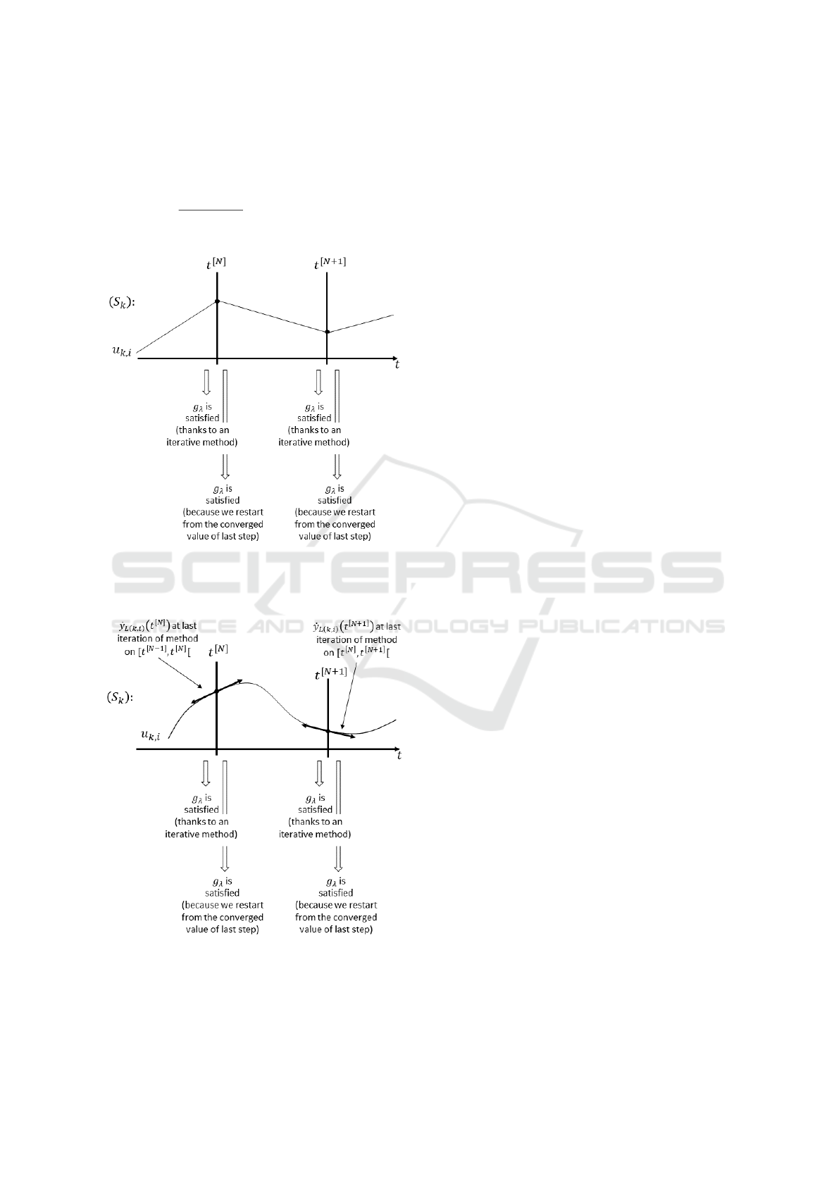
The idea of IFOSMONDI coupling is to use iter-
ative schemes so that the coupling constraint is sat-
isfied at the end of the current macro-step. More-
over, if this is done at every macro-step, using at least
1
st
order polynomial representation of the inputs may
keep this regard at the beginning of the step, and fur-
thermore avoid the introduction of discontinuities (see
figure 4). If additionally
ˆ
ˆ
S is available (see (11)), it is
possible to have C
1
inputs even while crossing com-
munication times with 3
rd
order Hermitian interpola-
tion polynomials (TOH) (see figure 5).
Due to conditionning issues that may appear on
small macro steps [t
[N]
,t
[N+1]
[, it may be necessary to
process the Hermite polynomial computation through
SIMULTECH 2019 - 9th International Conference on Simulation and Modeling Methodologies, Technologies and Applications
180
a variable change on [0, 1[. It implies a scaling on the
derivatives at t
[N]
and t
[N+1]
(respectively becoming
the derivatives at 0 and 1), but it may avoid failures
when t
[N]
>> 0 and t
[N+1]
− t
[N]
is very small (be-
cause of the
1
(
t
[N−1]
−t
[N]
)
2
factor in the coefficients of
the polynomial.
Figure 4: IFOSMONDI results on k
th
subsystem with FOH.
The drawn u are the one of the representation on last itera-
tion of iterative method for each macro-step.
Figure 5: IFOSMONDI results on k
th
subsystem with TOH.
The drawn u are the ones of the representation on last itera-
tion of iterative method for each macro-step.
3.2 Iterative Methods
IFOSMONDI offers two iterative methods that can al-
ternatively be chosen in order to ensure the coupling
condition (16) at the end of the macro-steps.
These iterative methods are Newton’s algorithm
and fixed-point method. Due to space concerns, the
Newton version of IFOSMONDI coupling will be de-
scribed in an extended version of this paper, still it can
be seen as a generalization of methods such as (Sick-
linger et al., 2014) or (Schweizer and Lu, 2015). Il
will be detailed in a further paper so that the analysis
can really be linked to (Sicklinger et al., 2014) and
(Schweizer and Lu, 2015).
Let t
[N]
be the N
th
discretization time. For the sake
of readability, we will write the global input vector (or
non-rectangular matrix) at the time t
[N]
as in (17).
u
[N]
:= (u
[N]
k,i
)
k∈[[1,n
sys
]]
i∈[[1,n
in,k
]]
(17)
Now, the assumption is that t
[N]
has been successfully
reached, and that the coupling condition is satisfied at
this time (18).
g
λ
u
[N]
= 0 (18)
The aim of an iterative method is to find u
[N+1]
=
(u
[N+1]
k,i
)
k∈[[1,n
sys
]]
i∈[[1,n
in,k
]]
so that the coupling condition is sat-
isfied at the left of t
[N+1]
, that is to say at the end of
the macro-step [t
[N]
,t
[N+1]
[.
g
λ
u
[N+1]
= 0 (19)
Let Ψ be defined as in (20).
Ψ :
R
n
in,tot
→ R
n
in,tot
u 7→ u − g
λ
u
n
in,tot
=
∑
n
sys
k=0
n
in,k
(20)
We can notice that
Ψ
u
= u ⇐⇒ g
λ
u
= 0 (21)
which means that (19) is equivalent to
Ψ
u
[N+1]
= u
[N+1]
(22)
that is to say
Ψ
(u
[N+1]
k,i
)
k∈[[1,n
sys
]]
i∈[[1,n
in,k
]]
= (u
[N+1]
k,i
)
k∈[[1,n
sys
]]
i∈[[1,n
in,k
]]
(23)
IFOSMONDI: A Generic Co-simulation Approach Combining Iterative Methods for Coupling Constraints and Polynomial Interpolation for
Interfaces Smoothness
181
It is thus possible to implement a fixed-point algo-
rithm to find (u
[N+1]
k,i
)
k∈[[1,n
sys
]]
i∈[[1,n
in,k
]]
. As an initial guess, it
is possible to use (u
[N]
k,i
)
k∈[[1,n
sys
]]
i∈[[1,n
in,k
]]
.
Let denote the fixed-point iteration by a left expo-
nent. We therefore set
∀k ∈ [[1, n
sys
]], ∀i ∈ [[1, n
in,k
]],
[0]
u
[N+1]
k,i
:= u
[N]
k,i
[m+1]
u
[N+1]
k,i
:=
Ψ
(
[m]
u
[N+1]
l, j
)
l∈[[1,n
sys
]]
j∈[[1,n
in,l
]]
!
k,i
(24)
Regarding the last line of (24), it is possible to sim-
plify the expression while using the definition of Ψ
(20) and g
λ
(15).
∀k ∈ [[1, n
sys
]], ∀i ∈ [[1, n
in,k
]],
[m+1]
u
[N+1]
k,i
:=
Ψ
(
[m]
u
[N+1]
l, j
)
l∈[[1,n
sys
]]
j∈[[1,n
in,l
]]
k,i
=
[m]
u
[N+1]
l, j
l∈[[1,n
sys
]]
j∈[[1,n
in,l
]]
− g
λ
[m]
u
[N+1]
l, j
l∈[[1,n
sys
]]
j∈[[1,n
in,l
]]
!
k,i
=
[m]
u
[N+1]
k,i
−
g
λ
[m]
u
[N+1]
l, j
l∈[[1,n
sys
]]
j∈[[1,n
in,l
]]
!
k,i
=
[m]
u
[N+1]
k,i
−
[m]
u
[N+1]
l, j
−
[m]
y
[N+1]
L(l, j)
l∈[[1,n
sys
]]
j∈[[1,n
in,l
]]
!
k,i
=
[m]
u
[N+1]
k,i
−
[m]
u
[N+1]
k,i
−
[m]
y
[N+1]
L(k,i)
=
[m]
y
[N+1]
L(k,i)
(25)
Please note that in the equation above (25),
[m]
y
[N+1]
L(k,i)
denotes the result of the simula-
tion of system (L(k, i))
1
with inputs worthing
[m]
u
[N+1]
(L(k,i))
1
, j
j∈[[1,n
in,(L(k,i))
1
]]
at the end of step
[t
[N]
,t
[N+1]
[.
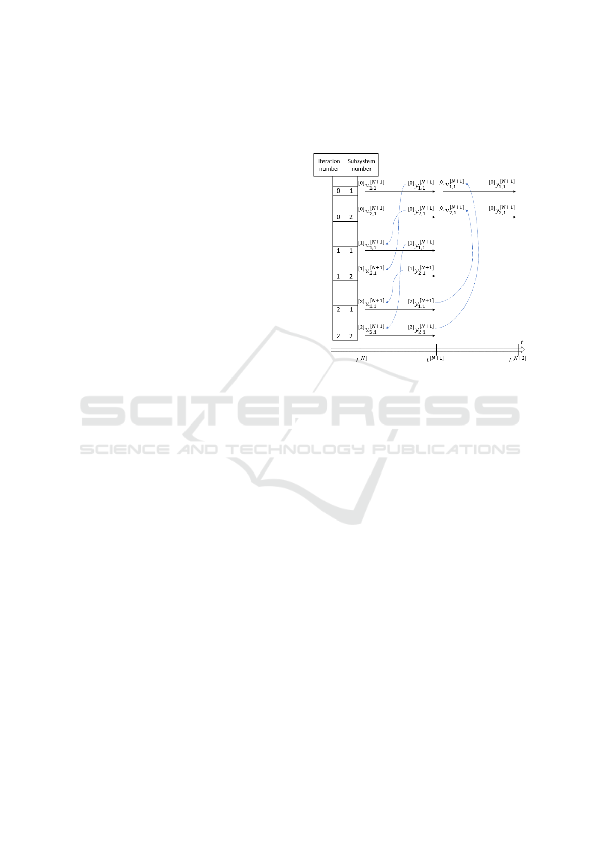
Consequently, if ZOH is used, the inputs of
subsystem (L(k, i))
1
have to be set to constant
[m]
u
[N+1]
(L(k,i))
1
, j
j∈[[1,n
in,(L(k,i))
1
]]
over the integration step
[t
[N]
,t
[N+1]
[ in order to produce
[m]
y
[N+1]
L(k,i)
and thus
[m+1]
u
[N+1]
k,i
. This way, smoothness cannot be re-
spected and it is impossible to get a satisfied coupling
constraint at left and right of every communication
time such as in figures 4 and 5, but we get at least
a satisfied coupling constraint at left of each of these
times as far as the fixed-point method converges. Fig-
ure 6 shows an example of this case on two subsys-
tems: it is exactly the iterative Jacobi co-simulation
scheme. When we want to force an input to worth a
value at the end of a macro-step, we inject it at the
beginning (as it is constant in ZOH): figure 6 indeed
shows [N + 1] exponents on inputs at time t
[N]
.
Figure 6: Jacobi scheme (IFOSMONDI with ZOH in fixed-
point mode) with supposed convergence of fixed-point
method after 3 iterations, on two subsystems with L(1, 1) =
(2, 1) and L(2, 1) = (1, 1).
As far as FOH is usable, it is possible to change
the scheme into a variant which is compliant with fig-
ure 4. Here are the steps :
• At t
[N]
, a converged value of
u
[N]
k,i
k∈[[1,n
sys
]]
i∈[[1,n
in,k
]]
is
known and satisfies the coupling constraint.
• We set ∀k ∈ [[1, n
sys
]], ∀i ∈ [[1, n
in,k
]],
[0]
u
[N+1]
k,i
:= u
[N]
k,i
.
• Until convergence, we integrate over [t
[N]
,t
[N+1]
[
with input i of system k represented by an affine
function worthing u
[N]
k,i
at t
[N]
and
[m]
u
[N+1]
k,i
at
t
[N+1]
.
This way, the first fixed-point iteration will necessar-
ily use ZOH, yet the following ones won’t. The cou-
pling condition reached at the end of [t
[N−1]
,t
[N]
[ will
not be broken at the beginning of [t
[N]
,t
[N+1]
[. More-
over, the continuity of the inputs will also be guaran-
teed since the fixed-point method converged on every
macro-step.
The principle can be extended to keep C
1
inputs
if time-derivatives of inputs can be obtained at the
end of every macro-step on every subsystem. TOH is
then used (Hermitian polynomial with 4 constraints).
In this case (corresponding to figure 5), the first
SIMULTECH 2019 - 9th International Conference on Simulation and Modeling Methodologies, Technologies and Applications
182
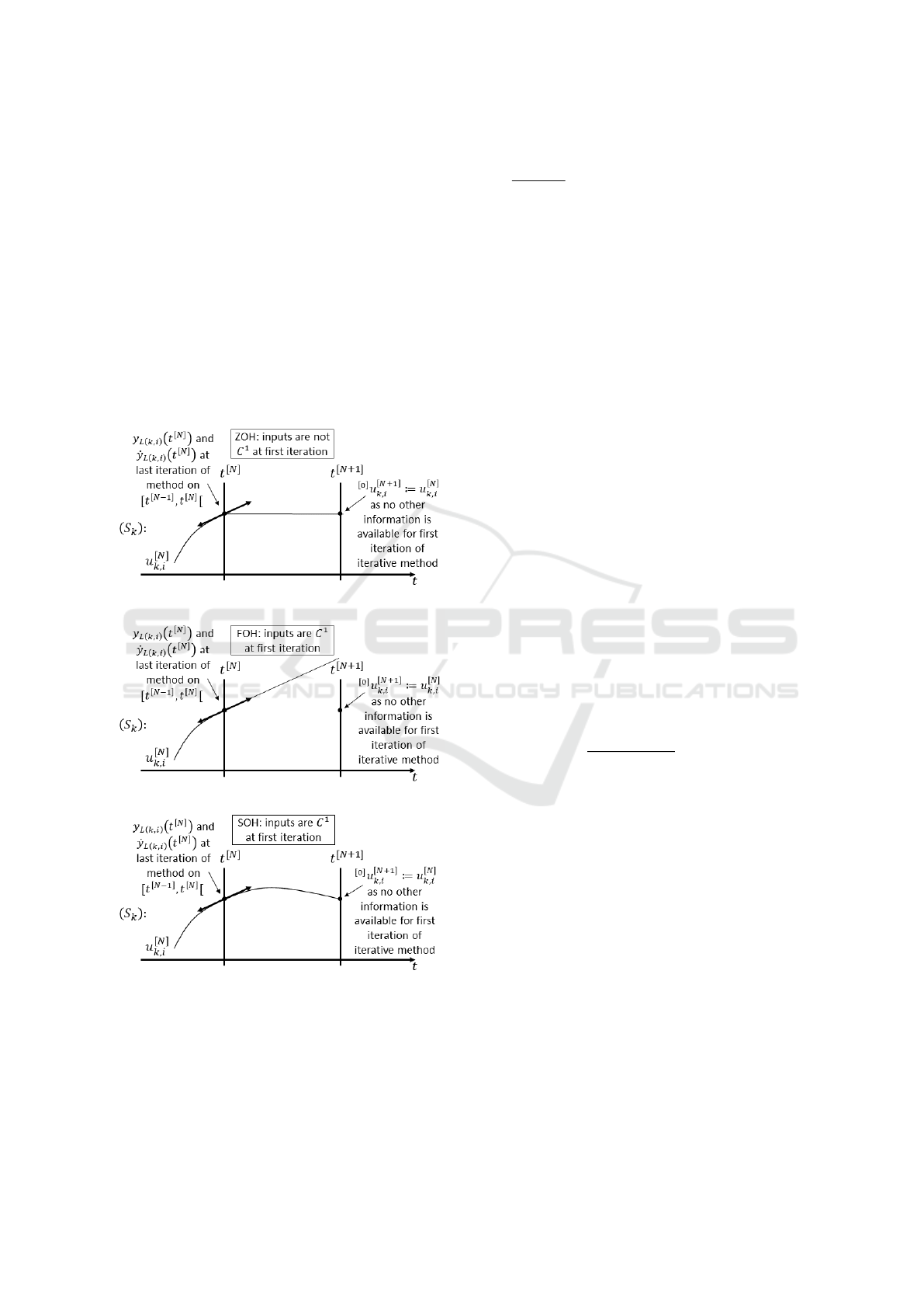
fixed-point iteration of every macro-step needs to be
smoother than ZOH in order to avoid time-derivative
continuity break. Indeed, figure 7 shows that at least
FOH should be used to keep C
1
inputs. However, us-
ing FOH at the first fixed-point iteration on a given
macro-step can only be done with extrapolation (as
no other information can be known), so the dangers
showed on figure 3 may appear. To reduce (but not an-
nihilate) the risk of out-of-range values, SOH (stand-
ing for second-order-hold) can be done by forcing the
polynomial to rejoin at the end of the macro-step the
value it had at the beginning.
Current implementation of IFOSMONDI cou-
pling uses SOH for first iteration of new macro-step
when TOH is used overall (to have C
1
inputs).
Figure 7: IFOSMONDI with TOH in fixed-point mode: vi-
sualisation of 3 strategies for first iteration of a new macro-
step following a converged one.
3.3 Step Size Control
When the fixed-point method does not converge af-
ter m
max
+ 1 iterations, it is possible to restart the
macro-step with reduced size (to try to integrate over
[t
[N]
,
t
[N]
+t
[N+1]
2
[ e.g.). However, this is not a real error-
based criterion of step-size adaptiveness. Such crite-
ria can be established for methods which allow esti-
mation of local error (Busch, 2016), yet here, IFOS-
MONDI coupling computes the fixed-point method
until convergence.
Researches about the use of such a criterion are
currently in progress. However, this paper only
presents fixed-step version of IFOSMONDI coupling.
The currently used rule-of-thumbs is:
• Define an initial synchronous macro-step size δt.
• Define m
max
, a maximum number of iterations to
reach (m should never exceed m
max
).
• At the beginning of any new macro-step, try to
integrate over a step of size min
δt, 1.3 δt
[N−1]
where δt
[N−1]
was the previous macro-step size
for which the iterative method converged.
• As soon as the iterative method converged, start
the next macro-step.
• If the iterative method does not converge, while m
reaches m
max
without convergence, divide δt by
two and restart from the last reached converged
time.
Further investigations will overwrite this rule. The
convergence of the iterative method is defined by a
criterion based on two values to provide: ε
abs
and
ε
rel
. For subsystem k ∈ [[1,n
sys
]] input i ∈ [[1, n
in,k
]],
the convergence is assumed when
|u
k,i
− y
L(k,i)
|
ε
rel
|u
k,i
| + ε
abs
< 1 (26)
The convergence of the iterative method on a macro-
step is assumed when every input has converged, that
is to say when
∀k ∈ [[1, n
sys
]], ∀i ∈ [[1, n
in,k
]],
|u
k,i
− y
L(k,i)
| < ε
rel
|u
k,i
| + ε
abs
(27)
When ε
abs
= ε
rel
, these values may be denoted by ε.
3.4 Algorithm
The fixed-point iterative method (subsection 3.2) is
used to satisfy the coupling constraint (subsection
3.1) defined in (16) (subsection 2.3) on a 2-side neigh-
borhood of each communication time. The macro-
step will be adapted until the fixed-point method con-
verges (subsection 3.3) on every macro-step. The
IFOSMONDI coupling combines all the previously
mentioned aspects. Its pseudo-code is given below.
IFOSMONDI: A Generic Co-simulation Approach Combining Iterative Methods for Coupling Constraints and Polynomial Interpolation for
Interfaces Smoothness
183
Algorithm 1 : IFOSMONDI coupling method in ”fixed-
point” mode for n
sys
∈ N
∗
subsystems.
Require: t
init
,t
end
initial and final times
δt base macro-step
(y
[0]
k
)
k∈[[1,n
sys
]]
initial outputs
(
ˆ
S
k
)
k∈[[1,n
sys
]]
simulation functions
L link function
ε
abs
, ε
rel
> 0 convergence criteria
m
max
iteration max
1: N := 0
2: t
[0]
:= t
init
3: δt
[0]
:= δt
4: ∀k ∈ [[1,n
sys
]], ∀i ∈ [[1, n
in,k
]], u
[0]
k,i
:= y
[0]
L(k,i)
5: while t
[N]
< t
end
do
6: t
[N+1]
:= t
[N]
+ δt
[N]
7: m = 1 interation of iterative method
8: while
m < m
max
∧
(27) is false
do
9: for k ∈ [[1, n
sys
]] do in parallel
10: if m = 1 then
11:
for every input,
build
[0]
u
[N]
as SOH in figure 7
12: else
13:
for every input, build
[m]
u
[N]
as TOH in figure 5
using
[m−1]
y
[N]
and
corresponding time-derivatives
14: end if
15:
(
[m]
y
[N]
k, j
)
j∈[[1,n
out,k
]]
:=
ˆ
S
k
(
t
[N]
t
[N+1]
,
(
[m]
u
[N]
)
k,i
i∈[[1,n
in,k
]]
)
16: end for
17: m ← m + 1
18: end while
19: if m = m
max
then convergence test failed
20: δt
[N]
←
δt
[N]
2
erase
21: else convergence test succeeded
22: δt
[N+1]
:= min
δt, 1.3 δt
[N]
23: N ← N + 1
24: end if
25: end while
4 RESULTS ON BENCHMARK
MODEL
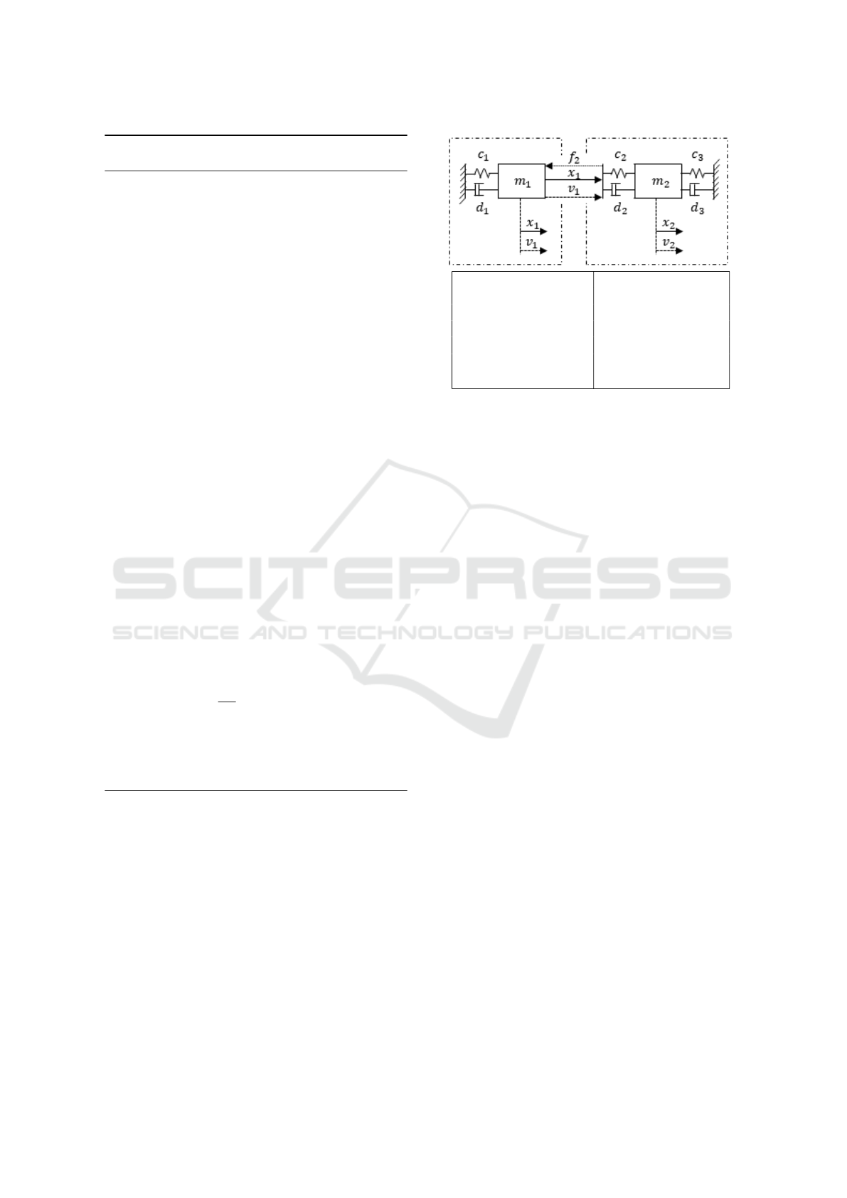
4.1 Benchmark Model
The model that will be considered is the two masses
oscillator (Busch, 2016) presented on figure 8 with the
chosen unbalanced parameters to avoid instantaneous
simulations, and to enable comparisons of execution
time.
c
1
= 1000 N/m d
1
= 10 N/(m/s)
c
2
= 1000 N/m d
2
= 10 N/(m/s)
c
3
= 100000 N/m d
3
= 0 N/(m/s)
m
1
= 1 kg m
2
= 1 kg
x
1
(t
init
) = −1 m x
2
(t
init
) = −3 m
v
1
(t
init
) = 0 m v
2
(t
init
) = 0 m
t
init
= 0 s t
end
= 100 s
Figure 8: Two masses model with coupling on force, dis-
placement and velocity and the chosen unbalanced parame-
ters.
Let the model of figure 8 be decoupled in two sub-
systems: the k = 1 denoting the left part (carrying
them mass m
1
) and the k = 2 denoting the right part
(carrying the mass m
2
). The interfaces are:
(S
1
) :
n
in,1
= 1
u
1,1
= f
2
n
out,1
= 2
y
1,1
= x
1
y
1,2
= v
1
(S
2
) :
n
in,2
= 2
u
2,1
= x
1
u
2,2
= v
1
n
out,2
= 1
y
2,1
= f
2
L(1, 1) = (2, 1)
L(2, 1) = (1, 1)
L(2, 2) = (1, 2)
(28)
4.2 Measures Environment
All measures have been made on the same virtual ma-
chine with 4 real cores. The co-simulations have been
launched one by one so that the performances of each
code were fully dedicated to the current processes.
Each co-simulation was made of 3 processes (1 for
each subsystem and 1 for the orchestrator).
Either the two subsystems and the monolithic
reference have been built with Simcenter Amesim,
embedding the LSODA internal variable step solver
(called for an integration on multiple micro-steps for
each evaluation of
ˆ
S
k
, see (10)) on a macro-step.
4.3 Results
Results are presented on tables 1 and 2 in order to
notice the benefits of combining the iterative method
and enhanced smoothness of interfaces.
SIMULTECH 2019 - 9th International Conference on Simulation and Modeling Methodologies, Technologies and Applications
184

Table 1: Results on 2 masses oscillator benchmark on non-
iterative methods: Explicit (denoting synchronous ZOH co-
simulation) and (Busch, 2016) in its C
0
configuration using
FOH for inputs.
δt Explicit
(Busch, 2016)
with C
0
interfaces
1 · 10
−5
0.1% 0.2%
1868s 1813s
5 · 10
−5
0.7% 0.9%
379s 378s
1 · 10
−4
1.2% 1.5%
203s 179s
5 · 10
−4
2.6% 2.8%
40s 36s
1 · 10
−3
3.2% 3.3%
18s 20s
5 · 10
−3
3.7% 3.7%
5.4s 5.1s
1 · 10
−2
3.7% 3.7%
3.9s 4.1s
5 · 10
−2
4.3% 9.0%
1.1s 1.4s
The algorithm denoted as ”Explicit” in table 1 is
the most used in the industry due to its strong link
between the needed accuracy and the macro-step size
δt. Indeed, target precision may be reached by reduc-
ing this macro-step size, however this substantially in-
creases the computation time.
Enhancing smoothness of the interface variables
by having C
0
inputs (Busch, 2016) leads to a similar
behavior.
The benefits on accuracy produced by the fixed-
point method of the second coupling algorithm pre-
sented in (K
¨
ubler and Schiehlen, 2000) enable to
reach higher precisions than non-iterative methods for
bigger macro-steps (see left column of table 2). How-
ever, IFOSMONDI coupling presents the lowest com-
putation time to reach the accuracy of 0.2% of mean
relative error: 7.6s. It should be noted that the macro-
step δt only gives a trend: indeed, it will not necessar-
ily stay constant as explained in subsection 3.3.
Nevertheless, when the macro-step becomes too
small
1
, the third-order polynomial inputs in the case
of IFOSMONDI coupling behave similarly to first-
order polynomial inputs in the case of (K
¨
ubler and
Schiehlen, 2000). The consequence is that the com-
putation time and accuracy reach the same values for
these methods (see first line of table 2). However, it
can be investigated to implement a smarter restart of
the internal solvers (with bigger micro-steps just af-
1
In this precise case, too small stands for: too small to
produce a significative difference between the first and third
order polynomials.
ter the communication times) on each subsystem in
the case where the C
1
smoothness of inputs is garan-
teed: this may lead to a smaller computation time on
IFOSMONDI coupling even with a small macro-step
(top-right case of table 2).
Finally, in the results presented above, the time-
derivative are computed at the end of each macro-step
with a least-square method where a decentered Taylor
method will be more appropriate. The latter will be
tackled in further papers.
Table 2: Results on 2 masses oscillator benchmark on iter-
ative methods: (K
¨
ubler and Schiehlen, 2000) (denoting its
second simulator coupling method with p
E
= 1) and IFOS-
MONDI coupling in fixed-point mode and using TOH to
have C
1
interfaces ; in each case, parameters are fixed to
ε
abs
= ε
rel
= 10
−3
and m
max
= 10.
δt
K
¨
ubler & al, 2000 IFOSMONDI
with p
E
= 1 for coupling
continuous interfaces algorithm
1 · 10
−3
0.1% 0.1%
27s 27s
5 · 10
−3
1.0% 0.2%
8.3s 7.6s
1 · 10
−2
3.7% 0.6%
6.0s 5.3s
5 CONCLUSIONS
The IFOSMONDI coupling algorithm allows a good
trade-off between accuracy and elapsed time by com-
bining iterative coupling method and smooth repre-
sentations of interface variables. It gives similar to
better results than each approach taken separately.t
Investigations on further enhancements are made
possible in a context where IFOSMONDI coupling
is used, both upstream and downstream. Upstream
in the sense of enhancements on computations of
data needed by IFOSMONDI, and downstream in the
sense of enhancements regarding technical aspects of
the subsystems. Regarding the upstream enhance-
ments, the way the time-derivative are computed (cur-
rently done with a least squares method, a more robust
implementation based on Taylor truncated develop-
ments is currently being integrated) can be cited. Re-
garding the downstream enhancements, we can point
a faster restart of embedded solvers inside of the sub-
systems (as mentionned in subsection 4.3) when C
1
smoothness of inputs is garanteed at the communi-
cation times: the latters no more have to be seen as
discontinuities by the solvers.
We limited our presentation to the fixed-point it-
erative coupling and in a further paper we will fo-
IFOSMONDI: A Generic Co-simulation Approach Combining Iterative Methods for Coupling Constraints and Polynomial Interpolation for
Interfaces Smoothness
185

cus on Newton’s iterative coupling with our mathe-
matical formalism. Moreover, this formalism allows
us to design a generically usable method covering
domain-specific methods such as (Schweizer and Lu,
2015) (originally deriving from a predictor-corrector
approach).
REFERENCES
Arnold, M. (2010). Stability of Sequential Modular Time
Integration Methods for Coupled Multibody System
Models. Journal of Computational and Nonlinear Dy-
namics, 5(3):031003.
Arnold, M. and Unther, M. G. (2001). Preconditioned Dy-
namic iteration for coupled differential-algebraic sys-
tems. Bit, 41(1):1–25.
Bartel, A., Brunk, M., G
¨
unther, M., and Sch
¨
ops, S. (2013).
Dynamic iteration for coupled problems of electronic
circuits and distributed devices. SIAM J. Sci. Comput.,
35(2):B315–B335.
Busch, M. (2016). Continuous approximation techniques
for co-simulation methods: Analysis of numerical sta-
bility and local error. ZAMM Zeitschrift fur Ange-
wandte Mathematik und Mechanik, 96(9):1061–1081.
Gomes, C., Thule, C., Broman, D., Larsen, P. G., and
Vangheluwe, H. (2018). Co-simulation : State of the
art. ACM Computing Surveys, 51(3):49:1—-49:33.
Gu, B. and Asada, H. H. (2004). Co-Simulation of Al-
gebraically Coupled Dynamic Subsystems Without
Disclosure of Proprietary Subsystem Models. Jour-
nal of Dynamic Systems, Measurement, and Control,
126(1):1.
K
¨
ubler, R. and Schiehlen, W. (2000). Two Methods of Sim-
ulator Coupling. Mathematical and Computer Mod-
elling of Dynamical Systems, 6(2):93–113.
Li, P., Meyer, T., Lu, D., and Schweizer, B. (2014). Nu-
merical stability of explicit and implicit co-simulation
methods. J, 10(5):051007.
Petridis, K. and Clauß, C. (2015). Test of Basic Co-
Simulation Algorithms Using FMI. Proceedings of
the 11th International Modelica Conference, Ver-
sailles, France, September 21-23, 2015, 118:865–872.
Schweizer, B., Li, P., and Lu, D. (2016). Implicit co-
simulation methods: Stability and convergence analy-
sis for solver coupling approaches with algebraic con-
straints. ZAMM Zeitschrift fur Angewandte Mathe-
matik und Mechanik, 96(8):986–1012.
Schweizer, B. and Lu, D. (2015). Predictor/corrector co-
simulation approaches for solver coupling with alge-
braic constraints. ZAMM Zeitschrift fur Angewandte
Mathematik und Mechanik, 95(9):911–938.
Sicklinger, S., Belsky, V., Engelman, B., Elmqvist, H., Ols-
son, H., W
¨
uchner, R., and Bletzinger, K.-U. (2014).
Interface Jacobian-based Co-Simulation. Interna-
tional Journal for Numerical Methods in Engineering,
98:418–444.
Skelboe, S. (1992). Methods for Parallel Integration of
Stiff Systems of ODEs. BIT Numerical Mathematics,
32(4):689–701.
Skelboe, S. and Zlatev, Z. (1997). Exploiting the natural
partitioning in the numerical solution of ODE systems
arising in atmospheric chemistry. Lecture Notes in
Computer Science (including subseries Lecture Notes
in Artificial Intelligence and Lecture Notes in Bioin-
formatics), 1196.
SIMULTECH 2019 - 9th International Conference on Simulation and Modeling Methodologies, Technologies and Applications
186
