Optimal Control to Limit the Propagation Effect of a Virus Outbreak on

a Network

Paolo Di Giamberardino and Daniela Iacoviello

Dept. Computer, Control and Management Engineering Antonio Ruberti, Sapienza University of Rome,

via Ariosto 25, 00185 Rome, Italy

Keywords:

Epidemic Modeling, Computer Virus, System Analysis, Optimal Control.

Abstract:

The aim of this paper is to propose an optimal control strategy to face the propagation effects of a virus

outbreak on a network; a recently proposed model is integrated and analysed. Depending on the speciﬁc

model caracteristics, the epidemic spread could be more or less dangerous leading to a virus free or to a virus

equilibrium. Two possible controls are introduced: a test on the computers connected in a network and the

antivirus. In a condition of limited resources the best allocation strategy should allow to reduce the spread of

the virus as soon as possible.

1 INTRODUCTION

The computer virus spread represents an important is-

sue since all the connected devices are susceptible of

being infected. A computer virus is a code that in gen-

eral can modify normal operations, as well as dam-

age ﬁles, and attack other computers. It can be trans-

mitted by downloading ﬁles from internet, by using

external devices, or by e-mails. The implications of

this threat involve the ﬁeld of Cyber Security, that has

been recently deﬁned as a game between defender and

attacker, (Karunanithi et al., 2018). Since the com-

puters and the internet connection are becoming more

and more widespread, a computer virus is able to dis-

rupt the productivity and cause billions of damages,

(Zhu and Yang, 2012); therefore, a large amount of

resources has been dedicated to blocking the spread

of viruses.

There are many analogies with diseases epidemic

spread and also the nomenclature is similar. The ba-

sic model is the SIR one, where S stands for suscep-

tible, indicating the subjects, in this case the comput-

ers, free from virus but that can be infected, I stands

for the set of all the computers infected and infectious

and R represents the set of all recovered computers.

The computer virus may have a latent period dur-

ing which the device, while being infected, is still not

able to infect other computers, (Peng et al., 2013);

the delay with which a virus breaks out is an im-

portant parameter to be taken into account when im-

plementing a control strategy. From the early 1980s

the problem of computer virus detection and removal

has been faced, taking into account the characteris-

tics of this kind of infection: the latency, the para-

sitism, the hiding and the infectiousness (Hu et al.,

2015). The modeling of the computers virus dynam-

ics can vary depending on the speciﬁc scenario con-

sidered that suggests a more or less complex par-

tition of the population. In the recent paper (Fa-

tima et al., 2018) a susceptible-latent-breakingout-

quarantine-susceptible computer virus dynamics is

proposed and implemented, showing the positive ef-

fects of the quarantine. The scenario considered in

this paper is similar to the one in (Xu and Ren, 2016);

the population of computers connected in a network

is partitioned into four classes. Besides the classes

of susceptible S and recovered R computers, that are

the devices not infected that can become infected and

those that can not get the infection respectively, there

are two classes of infected computers. The ﬁrst one,

E, is the most dangerous, since it is assumed that the

virus has not yet manifested itself but the computers

in this class can infect the devices they get in touch

with; the second class, I, contains the computers in-

fected and in which the virus has broken itself out.

This is a common condition that could include in-

fected e-mails or viruses that break out with a delay.

It appears important to become aware of the presence

of a virus as soon as possible, and successively to ap-

ply the suitable antivirus. This is the rationale for the

choices of the two strategies proposed: u

represents

the test to be performed on the computers which are

Di Giamberardino, P. and Iacoviello, D.

Optimal Control to Limit the Propagation Effect of a Virus Outbreak on a Network.

DOI: 10.5220/0008052804550462

In Proceedings of the 16th International Conference on Informatics in Control, Automation and Robotics (ICINCO 2019), pages 455-462

ISBN: 978-989-758-380-3

455

supposed free of virus, i.e. S and E, while u

repre-

sents the antivirus to be applied on the known infected

computers I, once the infection has broken out.

In this paper a variation of the model proposed in

(Xu and Ren, 2016) is introduced and analysed, by

considering the reproduction number and the possible

existence of virus equilibrium. Optimal control strate-

gies are proposed to face a possible epidemic spread.

The paper is organized as follows; Section 2 is divided

into three parts; in the ﬁrst two a new model describ-

ing the computer virus spread is analysed considering

the reproduction number, the equilibrium points and

their stability. In the third, the optimal control strategy

is proposed to allocate efﬁciently the limited available

resources. In Section 3 numerical results show the

plausibility of the model and the effectiveness of the

introduced actions. Conclusions and future develop-

ments are presented in Section 4.

2 MATERIALS AND METHODS

In this Section a new model of virus spread in a com-

puter network is described and analysed. The inspi-

ration is the model proposed in the paper in (Xu and

Ren, 2016); the total set of computers connected the

internet is partitioned into four classes: S, the com-

partment of susceptible computers: they are the un-

infected computers connected to the network; E, the

compartment of exposed computers: they are the in-

fected computers where all viruses are latent; I, the

compartment of infected computers: they are the in-

fected computers where all the viruses are currently

breaking out; R, the compartment of recovered com-

puters: they are the recovered computers that have run

the antivirus software.

It is assumed that new computers are connected to

the network with rate b; a susceptible computer in S,

when having a connection with a computer in the ex-

posed class E, can get the virus with rate β. As an ef-

fect, it can become infected, moving to I, with a prob-

ability p, or latent, moving to E, with a probability

1 − p. A latent computer virus breaks out with rate γ,

and the computers are removed from the net with rate

µ; moreover, it is possible that the virus is temporar-

ily suppressed with probability ε > 0. The proposed

model is a variation of the one in (Xu and Ren, 2016),

having modeled the infection interaction between sus-

ceptible and exposed computers by the term βSE and

not βSI; another difference is the impossibility for an

infected device to become recovered without an ex-

ternal control.

The control actions introduced in this paper to

limit the spread of a virus consist in a prevention cam-

paign u

, such as to induce people to test the condi-

tion and the vulnerability of their computer, and in

the antivirus action u

; they are weighted by σ

and

representing the unit cost efﬁciency. The virus test

is applied on all the susceptible computers in S and

its result inﬂuences the evolution of number of the ex-

posed computers. The proposed model completed by

the control actions is:

S = b − βSE − µS (1)

E = (1 − p)βSE + εI − (γ+ µ)E − σ

(

S + E

(2)

I = pβSE + γE − (ε + µ)I + σ

(

S + E

− σ

(3)

R = −µR + σ

(4)

The controls u

are assumed bounded:

0 ≤ u

(t) ≤ U

, i = 1, 2 (5)

being U

the corresponding possible maximum value

of u

. Obviously, all the state variables S, E, I and

R are non negative, representing the number of the

computers in the four identiﬁed different conditions;

then, the same must hold for the initial conditions

S(0) = S

≥ 0 E(0) = E

≥ 0

I(0) = I

≥ 0 R(0) = R

≥ 0 (6)

2.1 The Model Analysis

The proposed model is now analysed to understand its

dynamical behavior. Two related aspects are now con-

sidered; the determination of the equilibrium points

and the reproduction number. To determine the equi-

librium points, the equation (4) of the model is not

informative and therefore only the ﬁrst three are con-

sidered from now on. For sake of notation, the model

(1)–(3) is represented as follows:

X = f (X,U) (7)

with state X =







S E I



and control input U =





In (7), f =





, where the f

are the r.h.s. functions

of equations (1)–(3). The equilibrium points are de-

termined by assuming null the control inputs u

and

considering the equation f (X) = 0. One solution, that

can be referred as the disease free equilibrium, is



0 0



(8)

To determine the other equilibrium points, if they

exist, it is useful to introduce the auxiliary variable

Z = βE + µ; from f

= 0

S =

, (9)

ICINCO 2019 - 16th International Conference on Informatics in Control, Automation and Robotics

456

can be obtained, whereas from f

= 0 one has

I =

E(pβb + γZ)

Z(ε + µ)

(10)

Therefore, the existence of S and I as equilibrium

state components depends on the existence of E. By

substituting expressions (9) and (10) in f

= 0, one

obtains E = 0, the disease free equilibrium, and

Z =

bβ(ε + µ − pµ)

µ(ε + µ + γ)

(11)

By recalling the deﬁnition of Z, one obtains:

E =

b(ε + µ − pµ)

µ(ε + µ + γ)

−

µB

−

(12)

once

A = ε + µ(1 − p) B = ε + µ + γ (13)

are deﬁned. If E > 0, that is

µB

(14)

then a second equilibrium point is obtained:







µB

βA

µB

−

(bAβ−µ

B)(pµB+Aγ)

µBβA(µ+ε)







(15)

It is useful to connect the existence of the second equi-

librium point with the rate β at which computers be-

come infected. From (14) it can be deduced that if

β >

= β

(16)

then system (7) has two equilibrium points, X

and

; if β < β

, the solution is not feasible since the

components assume negative values; for β = β

the

two solutions X

and X

coincide. The value β

the bifurcation one.

Now local stability of the equilibrium points is in-

vestigated computing the Jacobian matrix of the sys-

tem

J =





−βE − µ −βS 0

(1 − p)βE (1 − p)βS − (γ + µ) ε

pβE pβS + γ −(ε + µ)





(17)

and evaluating it in X

and, if it exists, in X

. As far

as the point X

in (8) is concerned, the evaluation of

(17) gives

J(X

) =







−µ −β

0 (1 − p)β

− (γ + µ) ε

0 pβ

+ γ −(ε + µ)







(18)

One eigenvalue of (18) is clearly λ

= −µ; the

other two are the roots of the polynomial equation



(ε + γ + 2µ) − (1 − p)β



λ+

µ(ε + γ + µ) − β

(ε + µ(1 − p)) = 0 (19)

The two solutions, written as function of all the pa-

rameters appearing in the equation, do not allow an

easy analysis. However, once the bifurcation value

(16) is computed, it can be interesting to study the

sign of the roots of (19) in a neighbourhood of the bi-

furcation condition. The two coefﬁcients can be eval-

uated setting β = β

± δ, with 0 < δ  1. By using

the expression (16) for β

, as well as the notations in

(13), the polynomial equation (19) becomes



+ µ ∓ (1 − p)



λ+

∓(ε + µ(1 − p))

δ = 0 (20)

It can be noted that if β = β

− δ is considered, the

two coefﬁcients of (20) are

+ µ + (1 − p)

δ > 0 (21)

(ε + µ(1 − p))

δ > 0 (22)

Then, for the Descartes’ rule of signs, the two solu-

tions have negative real part and the equilibrium point

is locally asymptotically stable. Once β = β

+ δ is

assumed, the coefﬁcient (22) becomes

−(ε + µ(1 − p))

δ < 0 (23)

while the coefﬁcient of λ changes its sign as δ varies.

However, no matter what the sign of the coefﬁcient of

λ is: the polynomial equation has one positive and one

negative real solutions; consequently, the equilibrium

point X

results unstable. This behaviour follows

the classical case of generic epidemic spread: there

is a bifurcation condition which separates the case of

only one asymptotically stable equilibrium point, cor-

responding to the disease free condition, and the case

of two equilibria, one again the disease free condition

which becomes unstable, and the second equilibrium

point, corresponding to the so called endemic condi-

tion, locally asymptotically stable. Also in this case it

is possible to verify that the equilibrium point X

locally asymptotically stable, when it exists. Since the

conditions obtained are function of all the parameters

involved, their analytical expressions are quite com-

plicated and not useful to bring to clear conclusions.

In the numerical simulations, after the deﬁnition of

the parameters values, the cases β < β

and β > β

are veriﬁed and illustrated.

Optimal Control to Limit the Propagation Effect of a Virus Outbreak on a Network

457

2.2 The Reproduction Number

In epidemic spread the reproduction number R , as

recalled in (Driessche, 2002) and (Driessche, 2017),

is a useful parameter to describe the ability of an in-

fectious disease to invade a population. In this case

the population is the set of all computers connected in

the network and R is now evaluated by the next gen-

eration matrix. More precisely, from the dynamical

model (1)– (3), considering only the compartments

containing the infected subjects, the dynamical evolu-

tions (2) and (3) can be split into two parts, collected

in the two vectors:

K =



(1 − p)βSE

pβSE



Y =



(µ + γ)E − εI

(ε + µ)I − γE



The matrix K accounts for the rate of appearance of

new infections in the compartments E and I, whereas

Y describes the rate of other transitions between them.

Now, the jacobian of K and Y (with respect to E and

I) evaluated at the free disease equilibrium X

yields

respectively:

F =

(1−p)βb

pβb

V =



µ + γ −ε

−γ ε + µ



The next generation matrix is FV

−1

, that is:

−1

βb



(µ + ε)(1 − p) ε(1 − p)

p(ε + µ) pε



µ[(µ + γ)(ε + µ) − εγ]

The reproduction number is deﬁned as the spectral

radius of the matrix FV

−1

; in this case it is quite easy

to compute it, getting

R =

(ε + µ − pµ)βb

µ[(µ + γ)(ε + µ) − εγ]

Aβb

(24)

Following the classical deﬁnition of reproduction

number, when R < 1 the epidemic spread is charac-

terised by a low contagious effect which tends to keep

limited the number of infected units, asymptotically

going to the disease free equilibrium; in the cases of

R > 1 the number of infected machines grows, go-

ing asymptotically to an endemic condition where the

more R is great the more are the infected machines.

In the present case, comparing expression (24) with

(16), it is possible to ﬁnd the relationship

R =

(25)

between the reproduction number and the bifurcation

condition, so that R > 1 coincides with the condition

of existence of the second equilibrium point X

, (14).

2.3 The Optimal Control Problem

Solution

In the proposed model (1)–(4) two limited controls

are introduced, u

and u

, aiming at a fast virus de-

tection and a suitable antivirus action; with the ﬁrst

control the computers in the infected latent condition

(E) are detected, whereas with the second one the an-

tivirus allows the recovery of the infected computers

in I. The available resources are generally bounded,

from economic, logistic and practical point of view;

this implies the need of suitable allocation strategy.

In the similar contest of epidemic diseases, the natu-

ral framework to face efﬁciently the virus spread with

limited resources is the optimal control theory. A cost

index is introduced; the idea is to choose the control

in such a way that the total number of infected com-

puters (i.e. computers in E and in the I classes) is

minimized, taking into account the resources limita-

tions (5). For sake of notation, they are rewritten as

= −u

≤ 0 q

= u

− u

≤ 0

= −u

≤ 0 q

= u

− u

≤ 0

(26)

The proposed cost index that interprets the dis-

cussed need is:

J =



+ A

+ B



dt (27)

where A

and B

, i, j = 1, 2 are the weights of the

states, E and I, and of the controls u

and u

respec-

tively. The optimal control problem can be solved by

using classical techniques of calculus of variation; the

Hamiltonian function is deﬁned as:

H =



+ A

+ B



+λ

(t)F(X,U) (28)

where λ(t) =



(t) λ

(t)



is the costate.

The necessary conditions of optimality are given by:

= −

∂H

∂X

, λ

) = 0 i = 1, 2, 3 (29)

0 =

∂H

∂u

∑

k=1

∂q

∂u

, j = 1, 2 (30)

= 0, η

≥ 0, j = 1, . . . , 4 (31)

Note that in (29) the independence of q

, j =

1, ..., 4 from the state X has been used. By taking into

account the conditions (31) the possible 2

cases are

reduced to 4. By solving conditions (30) and taking

into account the constraints (26) (5), along with (29),

the optimal controls u

, i = 1, 2 are determined:

= max{min{

(λ

− λ

)σ

(S + E)B

, u

}, 0} (32)

ICINCO 2019 - 16th International Conference on Informatics in Control, Automation and Robotics

458

= max{min{

(λ

− λ

)σ

, u

}, 0} (33)

Note that the optimal controls require the solution

of the costate equations (29) in addition to the state

equation (7) with the initial conditions (6).

3 NUMERICAL RESULTS AND

DISCUSSION

In this Section, a numerical analysis is performed to

study the proposed computer virus spread model and

the optimal control strategies. For the choices of the

model parameters the value proposed in (Xu and Ren,

2016) are assumed:

b = 5; β = 0.15; µ = 0.3;

ε = 0.01; γ = 0.4 (34)

The initial conditions are set equal to



100 5 0 0



(35)

thus assuming a ”population” of 105 devices, among

which 5 are in the E condition of being infected and

infectious, without knowing it. The control period is

set equal to 10 unit of time.

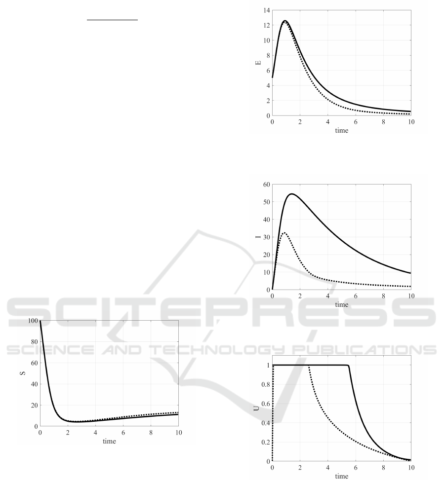
Figure 1: Case 1, β = 0.15: evolution of the number of sus-

ceptible computers (continuous line: free evolution; dotted

line: optimal control is applied).

Two cases are considered, depending on the value

of the probability p. As Case 1 it is chosen p = 0.8,

thus assuming that a computer, after being infected,

with high probability enters in the I class, meaning

that the infection is immediately known, and therefore

it can not infect other computers. With the chosen

values, R < 1 is obtained, thus meaning that only the

equilibrium point X

exists:



17 0 0 0



(36)

By evaluating the corresponding Jacobian (18) and its

eigenvalues, the stability of (36) can be veriﬁed. In

Figure 2: Case 1, β = 0.15: evolution of the number of

exposed computers (continuous line: free evolution; dotted

line: optimal control is applied).

Figure 3: Case 1, β = 0.15: evolution of the number of

infected computers (continuous line: free evolution; dotted

line: optimal control is applied).

Figure 4: Case 1, β = 0.15: evolution of the optimal control

strategies (continuous line: u

; dotted line: u

this case the parameters are such that for β = 0.15 it

results β

= 0.1826 and then β < β

, thus conﬁrming

that the system is below the bifurcation condition with

the chosen parameter values. By changing only the

value of β into 0.25, one gets β > β

and a completely

different situation it is obtained: R = 1.37 > 1 and

therefore also the second equilibrium point X

exists:



12 0 4 0



(37)

By considering the Jacobian (17) calculated in the two

Optimal Control to Limit the Propagation Effect of a Virus Outbreak on a Network

459

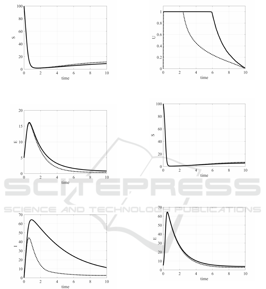
Figure 5: Case 1, β = 0.25: evolution of the number of sus-

ceptible computers (continuous line: free evolution; dotted

line: optimal control is applied).

Figure 6: Case 1, β = 0.25: evolution of the number of

exposed computers (continuous line: free evolution; dotted

line: optimal control is applied).

Figure 7: Case 1, β = 0.25: evolution of the number of

infected computers (continuous line: free evolution; dotted

line: optimal control is applied).

points X

, (36), and X

, (37), and evaluating the cor-

responding eigenvalues, one has that for X

the Ja-

cobian has one eigenvalue with positive real part, and

therefore it is unstable, while for X

all the eigen-

values have negative real parts, thus guaranteeing its

local asymptotic stability. These results conﬁrm what

has been previously stated in Section 2. The Case

2 regards the choice p = 0.2; this means that after

the infection most of the computers become laten; of

Figure 8: Case 1, β = 0.25: evolution of the optimal control

strategies (continuous line: u

; dotted line: u

Figure 9: Case 2, β = 0.15: evolution of the number of sus-

ceptible computers (continuous line: free evolution; dotted

line: optimal control is applied).

Figure 10: Case 2, β = 0.15: evolution of the number of

exposed computers (continuous line: free evolution; dotted

line: optimal control is applied).

course this is the most dangerous situation. In this

case β

= 0.051; by choosing β = 0.15, R = 2.53 > 1

is obtained. Therefore the second equilibrium point

exists and assumes the value



6 4 7 0



(38)

Since R > 1 the equilibrium point X

, given again

by (36), is unstable, as it can be veriﬁed by calculat-

ing the eigenvalues of (18), whereas the same analy-

sis applied to the second equilibrium point X

in (38)

ICINCO 2019 - 16th International Conference on Informatics in Control, Automation and Robotics

460

Figure 11: Case 2, β = 0.15: evolution of the number of

infected computers (continuous line: free evolution; dotted

line: optimal control is applied).

Figure 12: Case 2, β = 0.15: evolution of the optimal con-

trol strategies (continuous line: u

; dotted line: u

guarantees its stability.

If the parameter β is reduced to β = 0.015, that is

to a value lower than β

, R = 0.25 < 1 is obtained.

Therefore, a unique stable equilibrium point, X

, is

expected, as it can be directly veriﬁed by considering,

as usual, the eigenvalues of (18).

The optimal control actions are determined by

minimizing (27); the values A

= 10, A

= 0.1, B

= 1

and B

= 10 are chosen for the weights, whereas for

the boundaries (5) of u

and u

, u

= u

= 1 are as-

sumed. This means that the main aim is to minimize

the number of exposed computers, being the most

dangerous; therefore the limitations of the resources

in the cost index is less restrictive when referring to

the u

, rather than u

. In Figs. 1–3 the evolutions

of the state in Case 1 with the choice β = 0.15 are

shown; they are the effects of the optimal control de-

picted in Fig. 4, that proposes the maximum allowed

value 1 for u

up to about time 5.5, whereas the sec-

ond control u

must be at its maximum value up to

time 3. The effects of these controls are evident in the

almost halved number of infected, Fig. 3. As seen, the

same Case 1 analysed with β = 0.25 yields a differ-

ent kind of solution with two equilibrium points; the

evolutions of the state along with the optimal controls

are shown in Figs. 5–8. Due to the more dangerous

situation, the number of exposed and of the infected

devices in free evolution is signiﬁcantly higher than

in the previous case, Fig. 7, reaching for the infected

computers almost the peak of 65 computers versus 55

of the previous case; also the number of exposed com-

puters reaches higher value (16 versus 13) compen-

sated with the controls, Fig. 6. As far as the control

is concerned, in this case a larger effort, up to time

6, is requested for the control u

that at the end of

the control time 10 has not yet reached its minimum

allowed value; similar considerations can be applied

to the optimal control u

, that after keeping the maxi-

mum value up to time 3, it decreases without reaching

the minimum value at time 10.

In Case 2, after the infection, a larger number

of computers becomes exposed, being able to infect

other devices; it can be expected a stronger control

action to face this dangerous situation, see Fig. 12 in

case of β = 0.15: for the u

action, the maximum ef-

fort is required for almost all the time period, whereas

the maximum value for u

is required almost up to

time 4. The results are shown in Figs. 9–11. As ex-

pected, the number of infected computers increases

sensibly in absence of any action but the optimal con-

trol is able to face the spread, Fig. 11. The same Case

2 is analysed assuming β = 0.015; this means that

the virus is not so dangerous as in the previous case;

coherently, the optimal control does not require the

maximum value for both u

and u

, see Fig. 16: the

best action for u

is the maximum value up to time 7,

whereas for the control u

it is not required the maxi-

mum value. This is reasonable, since the epidemic is

not spreading and therefore there is not a great need

of anti–virus action. The reduced capability of the

virus to spread can be evidenced also noting that the

evolution of the susceptible devices does not vary sig-

niﬁcantly without and with the control, Fig. 13, being

the epidemic situation not so dangerous.

Figure 13: Case 2, β = 0.015: evolution of the number of

susceptible computers (continuous line: free evolution; dot-

ted line: optimal control is applied).

Optimal Control to Limit the Propagation Effect of a Virus Outbreak on a Network

461

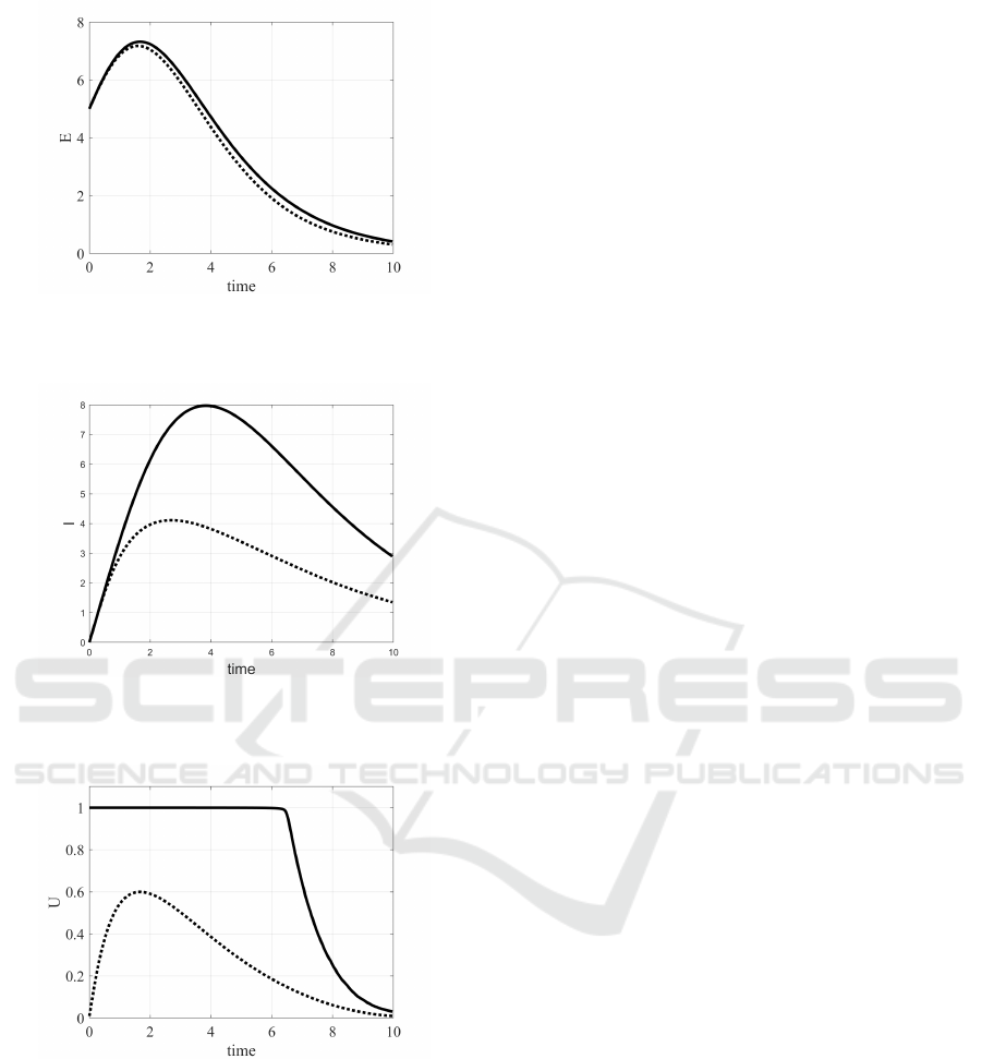
Figure 14: Case 2, β = 0.015: evolution of the number of

exposed computers (continuous line: free evolution; dotted

line: optimal control is applied).

Figure 15: Case 2, β = 0.015: evolution of the number of

infected computers (continuous line: free evolution; dotted

line: optimal control is applied).

Figure 16: Case 2, β = 0.015: evolution of the optimal con-

trol strategies (continuous line: u

; dotted line: u

4 CONCLUSIONS

The computer virus spread represents a problem in

a globalized world more and more connected, being

able to cause economic and social damages. By us-

ing the same modeling of epidemic disease spread, it

is possible to describe the dynamics of the computer

virus and to act in the most efﬁcient way, in order to

avoid as much as possible the obvious remedy, the

isolation of the infected computers. A simple dynam-

ical model to describe the computer virus spread is

proposed and optimal strategies are developed. The

ﬁrst results appear satisfactory and the effort will be

devoted to apply the discussed model and the control

scheme to a real scenario.

REFERENCES

Driessche, P. V. D. (2002). Reproduction numbers and

sub-threshold endemic equilibria for compartmental

models of disease transmission. Mathematical bio-

sciences, 18.

Driessche, P. V. D. (2017). Reproduction numbers of infec-

tious disease models. Infectious disease modelling, 2.

Fatima, U., Ali, M., Ahmed, N., and Raﬁq, M. (2018). Nu-

merical modeling of susceptible latent breaking-out

quarantine computer virus epidemic dynamics. He-

liyon, 4.

Hu, Z., Wang, H., Liao, F., and Ma, W. (2015). Stability

analysis of a computer virus model in latent period.

Chaos, Solitons and Fractals, 75(-):20–28.

Karunanithi, D., Alheyasat, O., Divya, T., and Kavitha, G.

(2018). Attacks on artiﬁcial intelligence applications

through adversarial image. International Journal of

Pure and Applied Mathematics, 118(20):4491–4495.

Peng, M., He, X., Huang, J., and Dong, T. (2013). Mod-

eling computer virus and its dynamics. Mathematical

Problems in Engineering, 2013.

Xu, Y. and Ren, J. (2016). Propagation effect of a virus

outbreak on a network with limited anti-virus ability.

PLOS ONE, October(27):1–15.

Zhu, Q. and Yang, X. (2012). Modeling and analysis of

the spread of computer virus. Commun. Nonlinear Sci

Numer Simulation, 17.

ICINCO 2019 - 16th International Conference on Informatics in Control, Automation and Robotics

462