Fault Diagnosis by Bayesian Network Classifiers with a Distance
Rejection Criterion
M. Amine Atoui
1
, Achraf Cohen
2
, Phillipe Rauffet
1
and Pascal Berruet
1
1
Lab-STICC, UMR 6285 CNRS, Universit
´
e Bretagne Sud, France
2
Department of Mathematics and Statistics, University of West Florida, Pensacola, Florida 32514, U.S.A.
Keywords: Bayesian Networks, Classification, Fault Diagnosis, Distance Rejection Criterion.
Abstract:
In this paper, Bayesian network classifiers (BNCs) are used as a statistical tool to diagnosis faults with a
distance rejection criterion. The proposed approach enhances significantly the structure of the use of Bayesian
networks in the same context. Our framework is evaluated and compared to state of the art using data from the
benchmark Tennessee Eastman Process (TEP).
1 INTRODUCTION
The existing monitoring techniques should always be
subject to improvement to deal with uncertainties and
complexities of modern systems. Therefore, develop-
ing novel fault diagnosis approaches has been a sig-
nificant research topic during the past decades. We
can find in the literature three main approaches, that
are a) data-driven approach, that is concerned with
the collected data from processes to develop a statis-
tical model for monitoring, b) knowledge-based ap-
proach that is based on experts, and c) model-based
approach that requires a prior physical and mathemat-
ical knowledge of the process.
The ultimate goal in fault diagnosis is to accu-
rately identity various types of faults that may affect a
process. Faults are commonly defined as changes ei-
ther in the mean vector or in the covariance matrix, or
both. This paper focuses on using Bayesian Networks
(BNs) as a framework with decision rules to diagnosis
and detect known and unknown faults.
BNs are powerful probabilistic tools. Previous
studies have proposed various networks for fault di-
agnosis. BNs have shown great abilities to fault di-
agnosis (Wang et al., 2019), (Jin et al., 2017), (He
et al., 2016), (Atoui et al., 2016), (Atoui et al., 2015b),
(Zhao et al., 2013), (Yu and Rashid, 2013), (Yang
and Lee, 2012). Though, one can observe from the
literature that the proposed BNs i) rely only on the
maximum posterior probability discrimination rule
to make decisions; ii) don’t consider the possibility
of occurrence of new observations belonging to un-
known faults/ operating conditions.
In this work, we will tackle the aforementioned is-
sues when dealing with BN for Fault diagnosis. We
shall propose a BN for fault diagnosis dealing with
unknown class of faults. This paper is organized as
follows: Section 2 briefly introduces the BN classi-
fiers. In section 3, we present the proposed frame-
work. Section 4 presents performances comparisons
using the classical TEP benchmark. Finally, in Sec-
tion 5, we give conclusions and outlooks of the further
directions.
2 BAYESIAN NETWORK
CLASSIFIERS
A Bayesian Network (BN) is a probabilistic graphical
model (Nielsen and Jensen, 2009). It consists of the
following:
• a directed acyclic graph G, G=(V, E), where V and
E are respectively its nodes’ and arcs’ sets,
• a finite probabilistic space (Ω, Z, p), with Ω a
non-empty space, Z a collection of the subspaces
of Ω and, p a probability measure (we use the
same notation for both probability distributions
and probability density functions. The meaning
will be clear from the context) on Z with p(Ω) =
1,
• a set of random variables X = X
1
, . . . , X
l
assigned
to V and defined on (Ω, Z, p), such that:
p(X
1
, X
2
, . . . , X
l
) =
l
∏
i=1
p(X
i
|pa(X
i
)) (1)
Atoui, M., Cohen, A., Rauffet, P. and Berruet, P.
Fault Diagnosis by Bayesian Network Classifiers with a Distance Rejection Criterion.
DOI: 10.5220/0008053304630468
In Proceedings of the 16th International Conference on Informatics in Control, Automation and Robotics (ICINCO 2019), pages 463-468
ISBN: 978-989-758-380-3
Copyright
c
 2019 by SCITEPRESS – Science and Technology Publications, Lda. All rights reserved
463

where pa(X
i
) is the set of parent nodes of X
i
in
G,
• a conditional distribution associate to each node,
given its parent nodes, describing probabilistic de-
pendencies between variables,
• calculations named inference, used given the
availability of a new evidence about one or sev-
eral variables represented by the nodes of G, to
update the network.
One particular form of Bayesian networks is the
Conditional Gaussian Network (CGN). Each CGN’s
node represents a discrete or Gaussian random vari-
able.
Gaussian nodes given their Gaussian parents fol-
low a Gaussian linear regression models with param-
eters depending on the values of their discrete par-
ents. Let’s consider a Gaussian node Y with discrete
parents pa
D
(Y) = {D
1
, . . . , D
d
} and Gaussian parents
pa
C
(Y) = {D
1
, . . . , D
c
}. Its conditional distribution
could be written as below for each value k
pa
D
(Y)
of its
discrete parents:
p(Y|Y
1
, . . . , Y
c
, k = N (µ
k
+ R
Y
1
k
Y
1
+ . . .
+R
Y
c
k
Y
c
;Σ
k
), k ∈ I
pa(Y)
(2)
where µ
k
and Σ
k
are respectively the mean and the
covariance matrix of Y given its discrete parents’s
value k. I
pa(Y)
is a set of Y’s discrete parents values.
R
Y
1
, . . . R
Y
c
are the regression coefficient associated
respectively to Y’s Gaussian parents Y
1
, . . . , Y
c
.
BNs and their ability to encode relationships be-
tween variables could be used naturally to solve clas-
sification problems; generally under the assumption
that the data are normally distributed.
D
D
C
1
. . . C
K
p(C
1
) . . . p(C
K
)
X
D X
C
1
X ∼ N (µ
C
1
;Σ
C
1
)
. . . . . .
C
K
X ∼ N (µ
C
K
;Σ
C
K
)
Figure 1: A basic CGN classifier.
Consider a new observation vector x of X ∈ R
m
and K different classes C
k
, i ∈ {1, . . . , K}. A basic
conditional Gaussian network classifier equivalent to
quadratic discriminant analysis, given in Figure 1,
will assign x to the class C
k
with the maximal a pos-
terior probability p(C
k
|x). The Maximum A Posterior
(MAP) rule, δ, can be written as follows:
δ : x ∈ C
k
∗
, where k
∗
= argmax
k=1,...,K
p(x|C
k
) (3)
Other discrimination rules, derived from (3), in re-
spect of the BN’s learned/ employed structure, can
be derived by making assumptions on classes’ covari-
ance matrices and using equation (3).
In this paper, we shall propose a new set of rules
to diganosis known faults and detect unknown faults
in respect of a distance rejection criterion.
3 FAULT DIAGNOSIS WITH
DISTANCE REJECTION
Fault diagnosis consists of acknowledging the pres-
ence of a fault in a system, and then identifying which
fault is it.
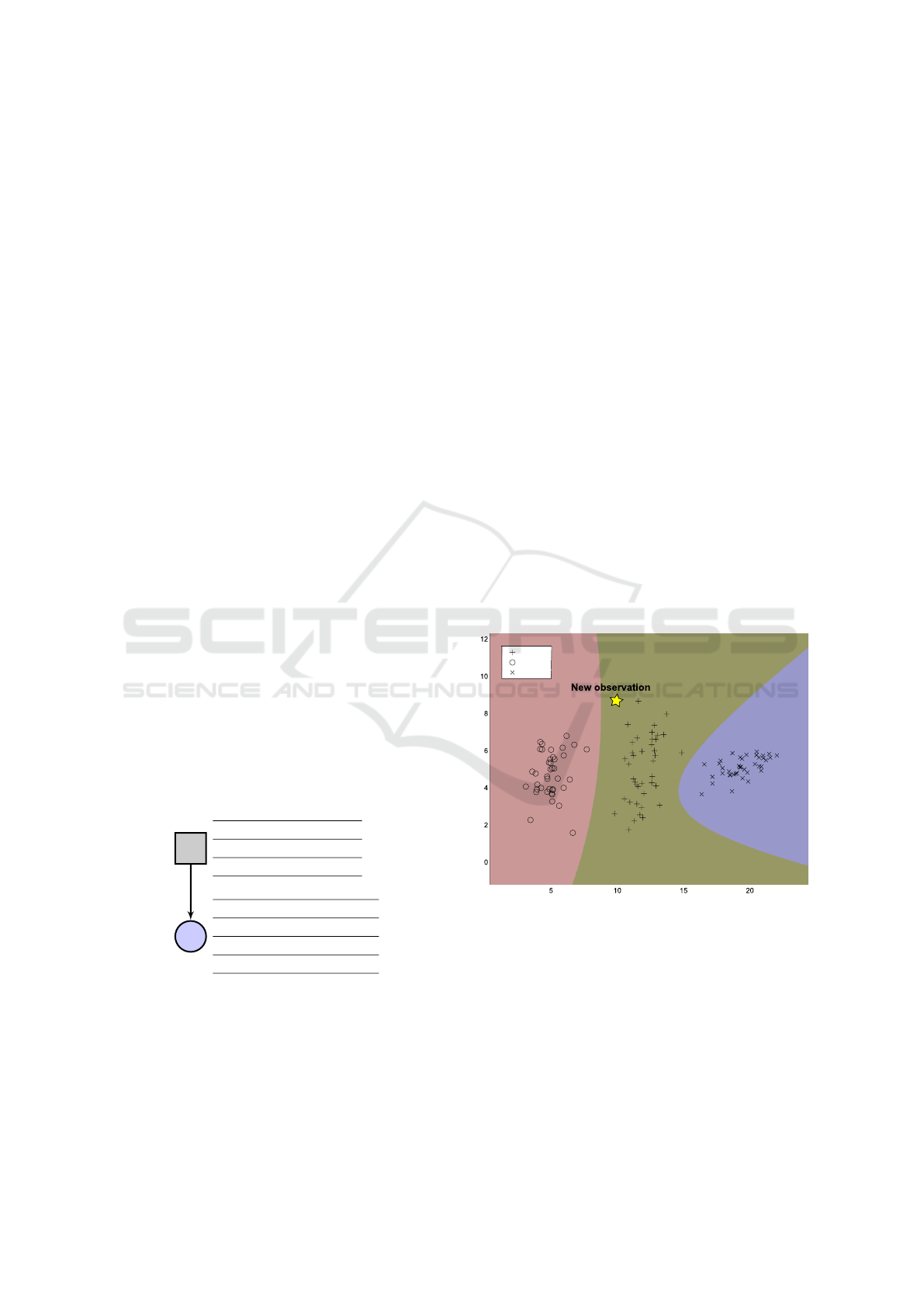
Fault diagnosis can be seen as a supervised clas-
sification problem. BNs can be used to define prob-
abilities boundaries between the faults’ classes (see
an example in Figure 2). Therefore, a new observa-
tion is assigned to the fault with the higher a poste-
riori probability. Though, under the assumption that
all the faulty operating conditions are known and well
defined.
Faults
Figure 2: BNC - quadratic discriminant analysis - decisions
discriminating between faults - standard approach.
However, in practice, it’s not obvious to describe
efficiently system’s faulty operating conditions. Also,
it is not always possible to identify the exact number
of possible faults that could influence/ change the sys-
tem from its normal operating conditions. Moreover,
it is hard to obtain/ collect enough data of faulty oper-
ating conditions that are rare or too risky to simulate.
Hence, it can be interesting to consider that some new
observations could do not belong to any of the exist-
ing/ known fault classes.
ICINCO 2019 - 16th International Conference on Informatics in Control, Automation and Robotics
464

A distance rejection criterion then can be used to
handle and consider a new unknown class in a BNC.
Thus, we propose a rule based on a new probabilis-
tic limit (more details are given in in the Appendix).
The proposed distance rejection criterion, given a new
observation x, compare the posterior probability of a
class C
k
∗
with the higher posterior probability to its
corresponding probabilistic limit, deduced from Ap-
pendix.(15) and given in (4), and decides statistically
based on a considered significance level α. It’s obvi-
ous α control the degree of exclusion, a higher value
of α would lead to shrinked ellipsoids and then more
exclusions.
PL
C
k
∆
=
τ
1 + e
−
1
2
(ϕ
1
−β
1
)
+ ·· · + e
−
1
2
(ϕ
K−1
−β
K−1
)
(4)
with
ϕ
j
= ∆
C
j
− ∆
C
k
, (5)
β
j
= 2ln(ω
j
|Σ
C
k
|
1
2
|Σ
C
j
|
1
2
), (6)
ω
j
=
p(D = C
j
)
p(D = C
k
)
(7)
where j = 1, . . . , K.
If p(C
k
∗
|x) > PL
C
k
∗
∆
then we classify an observa-
tion x as C
k
, else we attribute the observation to the
class UFC. Hence, we divide the decision space into
K + 1 sub-spaces (an example is shown in Figure 3),
where a new sub-space represents the class UFC, un-
known/ not defined states class. It’s clear that a BNC
following our approach isolate statistically each class
independently from the others classes. Basically, a
new observation is compared to the boundary associ-
ated to each class if it does not belong statistically to
any one of them then it belongs to the class UFC.
The following algorithm presents the steps we
propose to diagnose faults while incorporating a dis-
tance rejection criterion under BNCs.
Algorithm 1: Fault diagnosis with distance rejection crite-
rion.
Input: a new observation x
Outputs: the fault class to which x belongs
Calculate p(D = C
k
|x), for k ∈ 1, . . . , K
if p(D = C
k
∗
|x) ≥ PL
C
k
∗
∆
then
x ∈ C
k
∗
s.t. C
k
∗
= argmax p(C
ˆ
k
|x)
else
x ∈ UFC
 one can collect similar observations, define new
class and add it to the classifier
It worth noting to say that the proposed algorithm/
approach present a couple of advantages 1) it can be
Faults
Figure 3: BNC - quadratic discriminant analysis - decisions
discriminating between faults - our approach.
extended to handle multiple faults. We can do this
by testing statistically the belonging of a new obser-
vation to every class of fault instead of considering
the fault with highest posterior probability; 2) it can
be associated to several BN classifiers (e.g. PCA as
proposed in (Atoui et al., 2014)); 3) it can be easily
integrated and very useful to complex Bayesian net-
works such as the ones proposed by (Roychoudhury
et al., 2006), (Kawahara et al., 2005), (Schwall and
Gerdes, 2002) and (He et al., 2016); 4) it outperforms,
in the same context, the available approaches in terms
of time complexity and classification error rate as in
(Wang et al., 2017), (Verron et al., 2010). Further-
more, the number of the parameters and nodes is not
proportional to the number of faults; and 6) it can be
extended to detect and diagnosis known and unknown
faults, which we present in this paper.
4 PERFORMANCE AND
APPLICATION
In this section, we shall demonstrate and evaluate the
performance of the proposed approach using a com-
plex system: the Tennessee Eastman Process (TEP).
4.1 Presentation of the TEP
The Tennessee Eastman Process is a chemical pro-
cess. It is not a real process but a simulation of a pro-
cess that was created by the Eastman Chemical Com-
pany to provide a realistic industrial process in order
to evaluate process control and monitoring methods
(Downs and Vogel, 1993).
The TEP (flow sheet given on Figure 4) consists
of five major operation units: a reactor, a condenser, a
Fault Diagnosis by Bayesian Network Classifiers with a Distance Rejection Criterion
465

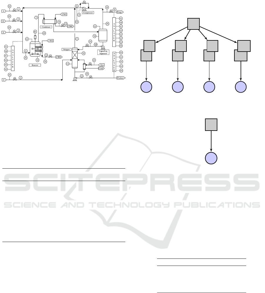
Figure 4: TEP flow sheet.
compressor, a stripper and a separator. Four gaseous
reactant A, C, D, E and an inert B are fed to the reactor
where the liquid products F, G and H are formed. This
process has 12 input variables and 41 output variables.
The TEP has 20 types of identified faults.
4.2 A BNC for Fault Diagnosis with a
Distance Rejection Criterion
Table 1: Description of datasets.
Class Fault type
Training
data
Test
data
F4
step change in the re-
actor cooling water inlet
temperature
480 800
F9
random variation in D
feed temperature
480 800
F11
reactor variation in the
reactor cooling water in-
let temperature
480 800
In the following, we shall compare the proposed ap-
proach to the one presented in (Verron et al., 2010) -
to our knowledge it is so far the most popular and effi-
cient method handling distance rejection in BNs’ state
of the art. The BN proposed by (Wang et al., 2017),
(Verron et al., 2010) is given in Figure 5. One can
notice its complex structure - five BNs (respectively
representing a quadratic discriminant analysis, three
control charts and a BN merging decisions). Indeed,
two inference phases are needed. These phases in-
volves the definition of several CPTs, transformation
of probabilities and many redundant inputs. Basically,
it depends on the number of faults which can lead to
a very complex and time consuming BN. We propose
to use a very simple BN structure presented in Figure
6, and representing, as an example, a quadratic dis-
criminant analysis (similarly to (Wang et al., 2017)
and (Verron et al., 2010)) associated to our proposed
algorithm.
D


F4
F9
F11


AD



F4
F9
F11
UFC



F4

Yes
No

F9

Yes
No

F11

Yes
No

D
F4
F9
F11
X X X X
Figure 5: The structure of the BN proposed by (Wang et al.,
2017) and (Verron et al., 2010).
D


F4
F9
F11


X
Figure 6: An example of a BNC’s structure - other BNC
could be considered - associated to our algorithm.
Consider now faults 4, 9 and 11 (see Table 6).
These faults are widely used in literature to compare
fault diagnosis methods. The three faults overlap,
making the classification task difficult. Several clas-
sifiers have been used to discriminate between these
faults. For instance, a learned BN classifier, equiva-
lent to a QDA, provide 18.75% as a misclassification
rate. More details are given in Table 2.
Table 2: Confusion matrix using the BN classifier without a
distance rejection criterion.
Class F4 F9 F11 Total
F4 659 0 141 800
F9 0 582 218 800
F11 28 66 706 800
Total 687 648 1065 2400
We tested both approaches on 7200 observations
(800 observations from respectively fault 4, 9, 11 and
4800 observations representing the class UFC (col-
lection of 800 observations from fault 7, 8, 10, 12, 13
and 14 (Chiang et al., 2012). The obtained results are
given in Tables 3 and 4.
From Table 4, the misclassification error rate ob-
tained by our approach, in respect to the 3 faults,
equals to 19.20 %, instead of 18.875% obtained by
a QDA. However, our approach outperforms the one
ICINCO 2019 - 16th International Conference on Informatics in Control, Automation and Robotics
466

Table 3: Confusion matrix using the BN integrating a dis-
tance rejection criterion proposed by (Verron et al., 2010).
C
k
F4 F9 F11 UFC Total
F4 654 0 144 2 800
F9 0 580 216 4 800
F11 28 65 695 12 800
UFC 132 122 194 4352 4800
Total 814 767 1249 4370 7200
proposed in (Verron et al., 2010) with a misclassifica-
tion error rate equals 19.62%, see Table 3.
Also, we can see that 4454 from 4800 observa-
tions belonging to the class UFC have been recog-
nized by our approach as unknown faults (miscclas-
sification error rate = 7.20%). Further, we have ob-
tained better performance, in respect to UFC, com-
pared with the the BN proposed in (Verron et al.,
2010), 9.33%.
We have shown how our new approach outper-
forms and can be an alternative to the state of the art.
Our approach is also able to simultaneously detect
and diagnosis simultaneously known and unknown
faults in a single Bayesian network.
Once again, the reader should notice that the re-
sults obtained by our approach depend considerably
on the used BN classifier. Obviously, several BNCs
can be associated to our proposal. The structure and
parameters of a given BNC are generally learned from
data. Different BNCs could be obtained in respect
of variables relationships and considered assumptions
(Friedman et al., 1997). BNCs are not only consid-
ered as powerful tools for classification but also as
frameworks for different data-driven fault diagnosis
schemes (Atoui et al., 2015a).
Table 4: Confusion matrix of an example of a BN classifier
integrating our distance rejection criterion.
C
k
F4 F9 F11 UFC Total
F4 655 0 141 4 800
F9 0 582 217 1 800
F11 28 65 702 5 800
UFC 0 132 214 4454 4800
Total 683 779 1274 4464 7200
5 CONCLUSIONS
In this paper, a new approach able to diagnosis faults
with a distance rejection criterion is proposed. Its per-
formances on the TEP gives excellent results com-
paratively to the literature. Obvious outlook of this
work is to expand our approach to simultaneously de-
tect and diagnose known and unknown faults. Also,
develop it for others data-driven BNCs to fault detec-
tion and diagnosis. Furthermore, it can be interesting
to enhance the decisions made by our approach by
considering different types of information.
REFERENCES
Atoui, M. A., Verron, S., and Abdessamad, K. (2014). Con-
ditional gaussian network as pca for fault detection.
IFAC Proceedings Volumes, 47(3):1935–1940.
Atoui, M. A., Verron, S., and Kobi, A. (2015a). Fault
detection and diagnosis in a bayesian network clas-
sifier incorporating probabilistic boundary1. IFAC-
PapersOnLine, 48(21):670–675.
Atoui, M. A., Verron, S., and Kobi, A. (2015b). Fault detec-
tion with conditional gaussian network. Engineering
Applications of Artificial Intelligence, 45:473–481.
Atoui, M. A., Verron, S., and Kobi, A. (2016). A bayesian
network dealing with measurements and residuals for
system monitoring. Transactions of the Institute of
Measurement and Control, 38(4):373–384.
Chiang, L., Russell, E., and Braatz, R. (2012). Fault De-
tection and Diagnosis in Industrial Systems. Springer
Science & Business Media.
Downs, J. J. and Vogel, E. F. (1993). A plant-wide indus-
trial process control problem. Computers & chemical
engineering, 17(3):245–255.
Friedman, N., Geiger, D., and Goldszmidt, M. (1997).
Bayesian network classifiers. Machine learning, 29(2-
3):131–163.
He, S., Wang, Z., Wang, Z., Gu, X., and Yan, Z. (2016).
Fault detection and diagnosis of chiller using bayesian
network classifier with probabilistic boundary. Ap-
plied Thermal Engineering, 107:37–47.
Jin, S., Liu, C., Lai, X., Li, F., and He, B. (2017). Bayesian
network approach for ceramic shell deformation fault
diagnosis in the investment casting process. The In-
ternational Journal of Advanced Manufacturing Tech-
nology, 88(1-4):663–674.
Kawahara, Y., Yairi, T., and Machida, K. (2005). Diag-
nosis method for spacecraft using dynamic bayesian
networks. In Proc. of 8th International symposium
on Artificial Intelligence, Robotics and Automation in
Space (i-SAIRAS). Citeseer.
Nielsen, T. D. and Jensen, F. V. (2009). Bayesian networks
and decision graphs. Springer Science & Business
Media.
Roychoudhury, I., Biswas, G., and Koutsoukos, X. (2006).
A bayesian approach to efficient diagnosis of incipi-
ent faults. In Proceedings of the 17th International
Workshop on Principles of Diagnosis (DX-06), pages
243–250. Citeseer.
Schwall, M. L. and Gerdes, J. C. (2002). A probabilistic
approach to residual processing for vehicle fault de-
tection. In Proceedings of the 2002 American Con-
trol Conference (IEEE Cat. No. CH37301), volume 3,
pages 2552–2557. IEEE.
Verron, S., Tiplica, T., and Kobi, A. (2010). Fault diagnosis
of industrial systems by conditional gaussian network
Fault Diagnosis by Bayesian Network Classifiers with a Distance Rejection Criterion
467

including a distance rejection criterion. Engineer-
ing applications of artificial intelligence, 23(7):1229–
1235.
Wang, J., Wang, Z., Stetsyuk, V., Ma, X., Gu, F., and Li, W.
(2019). Exploiting bayesian networks for fault isola-
tion: A diagnostic case study of diesel fuel injection
system. ISA transactions, 86:276–286.
Wang, Z., Wang, Z., He, S., Gu, X., and Yan, Z. F.
(2017). Fault detection and diagnosis of chillers us-
ing bayesian network merged distance rejection and
multi-source non-sensor information. Applied energy,
188:200–214.
Yang, L. and Lee, J. (2012). Bayesian belief network-
based approach for diagnostics and prognostics of
semiconductor manufacturing systems. Robotics and
Computer-Integrated Manufacturing, 28(1):66–74.
Yu, J. and Rashid, M. M. (2013). A novel dynamic
bayesian network-based networked process monitor-
ing approach for fault detection, propagation identi-
fication, and root cause diagnosis. AIChE Journal,
59(7):2348–2365.
Zhao, Y., Xiao, F., and Wang, S. (2013). An intelligent
chiller fault detection and diagnosis methodology us-
ing bayesian belief network. Energy and Buildings,
57:278–288.
APPENDIX
Assume each class C
k
, k = {1, . . . , K}, follow a nor-
mal distribution
x|C
k
:
1
2π
m
2
|S
C
k
|
1
2
e
−
1
2
(x−µ
C
k
)
T
S
−1
C
k
(x−µ
C
k
)
(8)
where m
C
k
and S
C
k
are respectively the mean and co-
variance of C
k
.
Let’s call ∆
k
the quadratic form associated to the
class C
k
∆
C
k
= (x − m
C
k
)
T
S
−1
C
k
(x − m
C
k
) (9)
The form ∆
k
based on its statistical distribution
(usually the chi-squared distribution is considered),
given significance level α, help to decide whether or
not a new observation belongs to the class C
k
. This is
done by comparing ∆ to its deduced limit CL
∆
(Con-
trol limit) as below
x ∈ C
k
, ∆
C
k
≤ CL
C
k
∆
(10)
By developing the inequality equation presented
above we obtain
x ∈ C
k
, if
∆
C
k
≤ CL
C
k
∆
−
1
2
∆
C
k
≥ −
1
2
CL
C
k
∆
e
−
1
2
∆
C
k
≥ e
−
1
2
CL
C
k
∆
p(x|D = C
k
) ≥ p(x
∗
|D = C
k
) (11)
where x
∗
is an observation of X with x
∗
∈ C
k
such as
∆
C
k
= CL
C
k
∆
.
Let’s multiply each side of (11) by p(x) as below
p(x)
p(x)
p(x|D = C
k
)p(D = C
k
)
≥ p(x
∗
|D = C
k
)p(D = C
k
) (12)
where
p(x) = p(x|D =C
1
)p(D = C
1
) + . . .
+ p(x|D = C
K
)p(D = C
K
) (13)
Thus, we deduce the following rule
x ∈ C
k
, if p(D = C
k
|x) ≥ PL
C
k
∆
(14)
with
PL
C
k
∆
=
p(x
∗
|D = C
k
)p(D = C
k
)
p(x)
(15)
It’s worth to mention that p(D = C
k
|x) corre-
sponds to the posterior probability of an observation
x given the value C
k
of the node D. The observation x
could concern one or several nodes.
ICINCO 2019 - 16th International Conference on Informatics in Control, Automation and Robotics
468