Sub-Sequence-Based Dynamic Time Warping

Mohammed Alshehri

1,2

, Frans Coenen

and Keith Dures

Department of Computer Science, University of Liverpool, Liverpool, U.K.

Department of Computer Science, King Khalid University, Abha, Saudi Arabia

Keywords:

Time Series Analysis, Dynamic Time Warping, k -Nearest Neighbor Classiﬁcation, Splitting Method.

Abstract:

In time series classiﬁcation the most commonly used approach is k Nearest Neighbor classiﬁcation, where

k = 1, coupled with Dynamic Time Warping (DTW) similarity checking. A challenge is that the DTW process

is computationally expensive. This paper presents a new approach for speeding-up the DTW process, Sub-

Sequence-Based DTW, which offers the additional beneﬁt of improving accuracy. This paper also presents an

analysis of the impact of the Sub-Sequence-Based method in terms of efﬁciency and effectiveness in compar-

ison with standard DTW and the Sakoe-Chiba Band technique.

1 INTRODUCTION

A time series is a set of sequentially recorded points

where each point references some numerical value;

examples include daily stock market prices (Chen and

Chen, 2015) or temperature recordings (Byakatonda

et al., 2018). Time series analysis is concerned with

the acquisition of an application speciﬁc understand-

ing of data. A common application domain is the clas-

siﬁcation of time series according to a predeﬁned set

of labels. The most frequently used time series classi-

ﬁcation technique is the k Nearest Neighbour (kNN)

technique with k = 1 (1-NN)(Tan et al., 2018; Silva

et al., 2018). Alternatives include Decision Trees

(Brunello et al., 2019), Artiﬁcial Neural Networks

and Support Vector Machines (SVM) (Agrawal and

Jayaswal, 2019).

When using kNN time series classiﬁcation, and

many other time series classiﬁcation techniques, the

choice of similarity measure to be used is a signif-

icant one. The criteria for selecting the most suit-

able distance measure depends on the nature of the

data (Rakthanmanon et al., 2012). In time series

data, to measure the similarity between two time se-

ries, Euclidean Distance is commonly used. How-

ever, alternatives have been found to be more effec-

tive. One of these alternatives is the Dynamic Time

Warping (DTW) technique (Silva et al., 2018; Tan

et al., 2018; Silva and Batista, 2016). The process

of DTW can be described as follows. Given two time

series, S

= [p

, p

,. .. , p

] and S

= [q

,. .. , q

where x and y are the lengths of S

and S

respec-

tively, a distance matrix M of size x × y is dynami-

cally constructed. The value held at each cell in M is

derived by applying a distance calculation to the as-

sociated points p

∈ S

and q

∈ S

using Equation 1,

where d

i, j

= |p

− q

| is the absolute difference be-

tween the value p

and q

. At the end of the pro-

cess the minimum warping distance (wd) will be held

at m

x,y

which in turn provides a similarity measure.

The minimum warping distance is associated with the

minimum warping path from m

0,0

to m

x,y

, which in

turn will approximate to the leading diagonal. Note

that if wd = 0 the two time series in question will be

identical and the minimum warping path will equate

to the leading diagonal. DTW offers the additional

advantage that the time series being compared do not

have to be of the same length, not the case when con-

sidering Euclidean distance similarity.

i, j

= d

i, j

+ min{m

i−1, j

i, j−1

i−1, j−1

} (1)

The computational complexity of DTW is given by

O(x × y). One of the challenges of DTW is thus that

the time complexity increases exponentially with the

size of the time series to be compared, an issue that is

compounded in the context of kNN time series classi-

ﬁcation which involves many comparisons. One way

of addressing this issue is to consider a subset of cells

in M deﬁned by a warping window, the cells located

near the leading diagonal where a “best” minimum

warping path is likely to exist. The nature of the warp-

ing window can be predeﬁned or learnt using training

data. The ﬁrst involves the user pre-specifying the

dimensions of the warping window and is the most

274

Alshehri, M., Coenen, F. and Dures, K.

Sub-Sequence-Based Dynamic Time Warping.

DOI: 10.5220/0008053402740281

In Proceedings of the 11th International Joint Conference on Knowledge Discovery, Knowledge Engineering and Knowledge Management (IC3K 2019), pages 274-281

ISBN: 978-989-758-382-7

straight forward; the dimensions are often referred to

as global constraints (global constraints on the mini-

mum warping path generation process). Examples in-

clude the Sakoe-Chiba band (S-C Band) (Sakoe and

Chiba, 1978) and the Itakura parallelogram (Itakura,

1975).

Table 1: Symbol Table.

Symbol Description

p or q A point in a time series described by a single value.

S A time series such that S = [p

, p

,...] or S = [q

,...].

x or y The length of a given time series.

M A distance matrix measuring x × y.

i, j

The distance value at location i, j in M.

W P A warping path [w

,...] where w

∈ M.

wd A warping distance derived from W P.

` the band width of a warping window (for the Sakoe-Chiba band).

α A warping window such as that generated using the Sakoe-Chiba

band.

s A number of sub-sequences into which a given time series is split.

C A set of class labels C = {c

,...}.

D A collection of time series {S

,..., S

}

r The number of time series in D.

z The runtime (secs.) to process a single point p in the context of DTW.

The idea presented in this paper, instead of consid-

ering the time series to be compared in their entirety,

is to split the time series into s sub-sequences and

to compare the sub-sequences. The time complexity

then decreases from O(x × y) to O(

x×y

). The ques-

tions to be answered then are: (i) does this retain an

adequate level of accuracy? And (ii) how should s be

deﬁned? This paper explores both these questions in

the context of 1-NN classiﬁcation coupled with stan-

dard DTW, and coupled with DTW applied only over

a “warping window” (the Sakoe-Chiba band). The

presented analysis was conducted using 10 different

time series datasets taken from the UEA and UCR

(University of East Anglia and University of Califor-

nia Riverside) Time Series Classiﬁcation Repository

(Bagnall et al., 2017).

The rest of this paper is organised as follows. A

review of previous work is presented in Section 2.

The operation of the proposed Sub-Sequence-Based

DTW method is then presented in Section 3 followed

by brief a description of kNN (1NN) time series clas-

siﬁcation in Section 4. The theoretical computa-

tional complexity of the proposed approach is then

discussed in Section 5. The evaluation of the pro-

posed approach is presented in Section 6. The paper

is concluded in Section 7. For convenience, a sym-

bol table is given in Table 1 listing the symbols used

throughout this paper.

2 PREVIOUS WORK

This section presents a review of previous work that

has been conducted to speed up DTW. Previously pro-

posed techniques have mostly been directed at limit-

ing the number of distance matrix values to be cal-

culated by deﬁning a “warping window” α such that

α ⊆ M. In other words, by placing constraints on the

matrix area to be considered when calculating a min-

imum warping path. These techniques can be cate-

gorised as follows:

1. Predeﬁned: Techniques where the nature of the

warping window is predeﬁned using one or more

parameters (global constraints).

2. Learnt: Techniques where the nature of the warp-

ing window is learnt using training data.

The use of a warping window α thus deﬁnes a con-

strained area inside the matrix M for which cell val-

ues need to be calculated. In addition, it prevents any

pathological alignment by forcing the warping path to

remain inside the constrained warping window area.

2.1 Predeﬁnition

The simplest mechanism for predeﬁning a warping

window is to deﬁne a band, of width `, stretch-

ing from m

0,0

to m

x,y

(given two time series S

, p

,. .. , p

] and S

= [q

,. .. , q

]). From the

literature the most well-documented example of this

approach is the Sakoe-Chiba band (Sakoe and Chiba,

1978), originally introduced and used by the speech

analysis community. In (Sakoe and Chiba, 1978) it

was suggested that that the value for ` deﬁning the

band width should be set to 10% of the time series

length.

An alternative to using a warping window in the

shape of a band is to use a parallelogram thus avoid-

ing unnecessary calculation at the start and end of the

warping path. The best-known example of this is the

Itakura parallelogram where the warping window α is

deﬁned by two slope constraints (Itakura, 1975). The

Sakoe-Chiba band and the Itakura parallelogram are

illustrated in Figure 1.

Figure 1: Left: The Sakoe-Chiba band, Right: The Itakura

Parallelogram (Niennattrakul and Ratanamahatana, 2009).

2.2 Learning

The predeﬁnition of a warping window requires the

user to, more-or-less, guess at the required deﬁni-

tion of the window; users thus tend to err on the

Sub-Sequence-Based Dynamic Time Warping

275

side of caution. A more accurate way of deﬁning

the warping window is to use a machine learning ap-

proach, although this requires training data. The idea

of learning the nature of the warping window was

ﬁrst proposed in (Niennattrakul and Ratanamahatana,

2009) in the context of time series classiﬁcation. The

idea here was to produce an arbitrarily shaped win-

dow. This was deﬁned by considering each class in

the training set in turn and identifying the minimum

warping path for each pair of time series subscribing

to that class. The collected warping paths for each

class then deﬁned warping sub-windows which were

then merged to deﬁne a global warping window. The

approach is illustrated in Figure 2 where the training

set features three classes (red, blue and green) whose

associated warping sub-windows are merged to form

a global window.

Figure 2: Warping Window learning example using three

individual classes (red, blue, green) (Niennattrakul and

Ratanamahatana, 2009).

3 SUB-SEQUENCE-BASED DTW

In this section the proposed Sub-Sequence-Based

DTW mechanism is presented. The proposed pro-

cess is similar to the fundamental (standard) DTW

process; the only difference is the splitting of the

time series into sub-sequences. Thus given two

time series S

and S

these are divided into s sub-

sequences so that we have S

= [U

,. ..U

] and

= [U

,. ..U

]. DTW is then applied to each

sub-seqence paring U

where i = j. The ﬁnal

minimum warping distance arrived at will be the ac-

cumulated warping distance for all sub-sequences af-

ter s application of DTW. There are two mechanisms

whereby s can be deﬁned:

1. Fixed Number: Directly by specifying a value

for s, a number of sub-sequences.

2. Fixed Length: In terms of a predeﬁned sub-

sequence length len, such that s =

len

, where x is

the length of the two time series to be compared

(assuming they are of equal length).

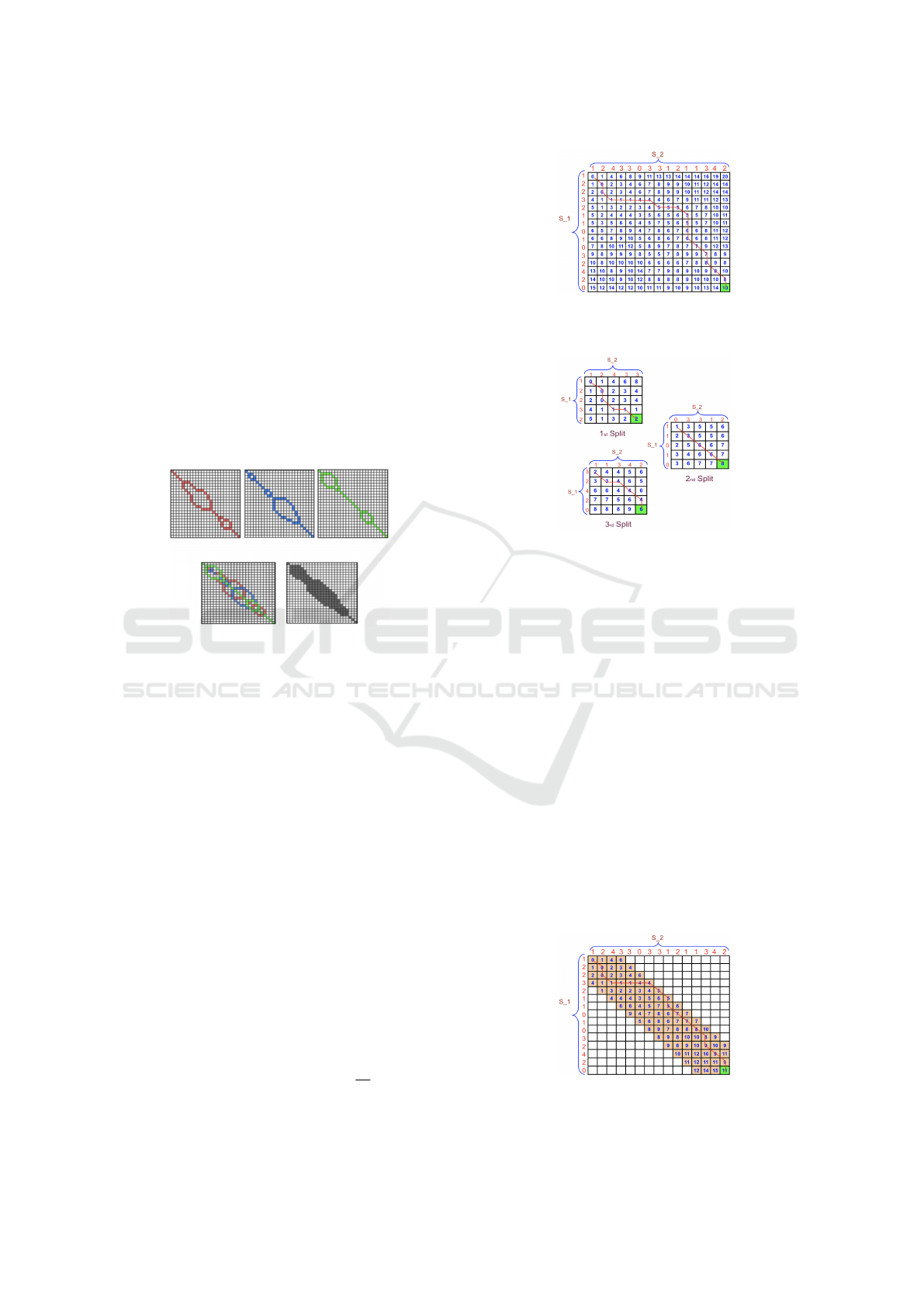
Figure 3: Distance Matrix and Warping Path (red line) for

the example time series S

and S

generated using standard

DTW.

Figure 4: Distance Matrices and Warping Paths (red lines )

for the example time series S

and S

generated using the

Sub-Sequence-Based method (s = 3).

Considering two time series, S

= [1,2,

2,3, 2, 1, 1, 0, 1, 0, 3, 2, 4, 2, 0] and S

= [1, 2, 4, 3, 3, 0,

3,3, 1, 2, 1, 1, 3, 4, 2], using standard DTW the ma-

trix M will measure 15 × 15 (the lengths of the

two time series); Figure 3 shows the distance

matrix. However; in case of the Sub-Sequence-

Based method the ﬁrst step is to deﬁne the

number of splits s. Assuming s = 3 there will

be three sub-sequences in each time series, S

1,1

1,2

] = [[1, 2, 2, 3, 2], [1,1, 0,1, 0],[3, 2, 4,

2,0]] and S

= [U

2,1

2,2

] = [[1,2,4, 3, 3], [0, 3,

3,1, 2], [1, 1, 3, 4, 2]]. Figure 4 shows the three result-

ing distance matrices. Figure 5 shows the resulting

distance matrix using a Sakoe-Chiba band warping

window when sub-sequence splitting is not used, and

Figure 6 when sub-sequence splitting is used, with

respect to the same example data. Where the green

cell presents the value of the warping distance wd.

Figure 5: Distance Matrix and Warping Path (red line) for

the example time series S

and S

generated using standard

DTW coupled with a Sakoe-Chiba band warping window.

KDIR 2019 - 11th International Conference on Knowledge Discovery and Information Retrieval

276

Figure 6: Distance Matrices and Warping Paths (red lines

) for the example time series S

and S

generated using

the Sub-Sequence-Based method (s = 3) and a Sakoe-Chiba

band warping window.

4 K-NN TIME SERIES

CLASSIFICATION

In time series classiﬁcation the most appropriate clas-

siﬁcation technique to be adapted depends on the na-

ture of the data (Rakthanmanon et al., 2012). As

noted earlier in this paper, k-nearest neighbour clas-

siﬁcation is the most common technique used in time

series classiﬁcation; k = 1 is most frequently used

(Silva et al., 2018; Tan et al., 2018; Silva and Batista,

2016).

The fundamental idea of kNN (1NN) classiﬁca-

tion is to use pre-labelled data as a data bank (a data

repository) D, comprised of r examples each asso-

ciated with a class c taken from set of class labels

C = {c

,. .. }. A new time series to be labelled

is then compared with every time series in D and the

labels associated with the k most similar time series

used to label the new time series. Where k > 1 there is

a possibility of conﬂict, in which case a conﬂict reso-

lution mechanism, such as voting, is required. Where

k = 1 this issue does not arise. Further detail concern-

ing the k-NN algorithm can be found in (Singh et al.,

2016).

5 TIME COMPLEXITY

From the foregoing the time complexity for compar-

ing two time series using standard DTW was given

by O(x × y). However, in most 1NN applications

the time series to be considered are all of the same

length, in which case the standard DTW time com-

plexity (DTW

complexityStand

) can be expressed as:

DTW

complexityStand

= O



× z



(2)

where z is a constant describing the time complexity

associated with a single cell m

i, j

in the distance ma-

trix M. The time complexity, when standard DTW is

combined with the Sakoe-Chiba band warping win-

dow (DTW

complexityStand+SC

), using the proposed sub-

sequence-based mechanism (DTW

complexitySplit+SC

)

and the proposed mechanism with the Sakoe-Chiba

band warping window (DTW

complexitySplit+SC

) can be

expressed as follows:

DTW

complexityStand+SC

= O



100

× z



(3)

DTW

complexitySplit

= O



× z



(4)

DTW

complexitySplit+SC

= O

100

× z

(5)

If we have a data repository with r examples the

time complexity to classify a single record using 1NN

is given by:



r × DTW

complexity



(6)

If there are t new time series to be classiﬁed (t > 1)

the complexity is given by:



r × DTW

complexity

×t



(7)

In the case of cross-validation, as presented in the fol-

lowing section, the complexity becomes:



r × DTW

complexity

×t × numFolds



(8)

When using ten cross validation the data set D is split

into tenths, in which case r =

9×|D|

, t =

|D|

and the

number of fold will equal 10:



9 × |D|

× DTW

complexity

|D|

× 10



(9)

Which simpliﬁes to:



9 × |D|

100

× DTW

complexity



(10)

6 EVALUATION

The evaluation of the proposed Sub-Sequence-Based

DTW is presented in this section. The evaluation was

conducted using 1NN classiﬁcation and ten selected

datasets from the UEA and UCR Time Series Classi-

ﬁcation repository (Bagnall et al., 2017). Further de-

tail concerning the data sets used for the experiments

is given in Sub-section 6.1 below. Experiments were

Sub-Sequence-Based Dynamic Time Warping

277

Table 2: Time Series Datasets Used for Evaluation Pur-

poses.

ID No. Dataset Length (x) No. records (r) Size x r No. Classes Type

1 GunPoint 150 200 30000 2 Motion

2 OliveOil 570 60 34200 4 Spectro

3 Trace 275 200 55000 4 Sensor

4 ToeSegment2 343 166 56938 2 Motion

5 Car 577 120 69240 4 Sensor

6 Lightning2 637 121 77077 2 Sensor

7 ShapeletSim 500 200 100000 2 Simulated

8 DiatomSizeRed 345 322 36000 4 Image

9 Adiac 176 781 137456 37 Image

10 HouseTwenty 2000 159 318000 2 Image

conducted using: (i) Standard DTW, the benchmark

approach (Standard DTW); (ii) DTW coupled with

time series splitting (Subsequence DTW); (iii) Stan-

dard DTW coupled with the Sakoe-Chiba band warp-

ing window (Standard DTW + SC) and (iv) DTW

coupled with time series splitting and the Sakoe-

Chiba band warping window (Subsequence DTW +

SC). To deﬁne the Sakoe-Chiba band, ` = 10% was

used as proposed in (Sakoe and Chiba, 1978).

The objectives of the evaluation were:

1. To determine the most suitable mechanism for

selecting a value for s (ﬁxed number or ﬁxed

length).

2. To evaluate the run-time advantages gained using

the time series Sub-Sequence-Based approach.

3. To determine whether the classiﬁcation accuracy

of the proposed approach was commensurate with

that obtained using standard DTW.

The ﬁrst two are considered in Sub-section 6.2 and the

third in Sub-section 6.3. Ten Cross Validation (TCV)

was adopted throughout (Roberts et al., 2017). For

the experiments, a desktop computer with a 3.5 GHz

Intel Core i5 processor and 16 GB, 2400 MHz, DDR4

of primary memory was used. The evaluation metrics

collected comprised run time (seconds), and accuracy

and the F1-score; the later derived from a confusion

matrix (Deng et al., 2016). The values reported later

in this section are average values, collected with re-

spect to each “fold” of the TCV, together with stan-

dard deviation values to indicate the “spread” of the

results obtained.

6.1 Data Sets

This section presents a brief overview of the data sets

used for the DTW analysis presented in this section.

In total ten datasets were downloaded from the UEA

and UCR repository. These were selected so that a

mix of datasets was obtained in terms of number of

points, number of records, number of classes and the

nature (type) of the data sets. An overview of the

ten data sets is given in Table 2. Column ﬁve, x × r,

gives an indication of the overall size of each dataset,

a measure referenced later in this section. The “Type”

of the data set describes the nature of the data set; the

terminology used is that used with respect to the UEA

and UCR repository (Bagnall et al., 2017). Sensor

data is time series data obtained by some form of sen-

sor such as an electric power signal sensor. Motion

data is time series data describing some of the body

motion. Spectro data is time series data collected us-

ing a spectrograph. Image data is time series data

collected through some boundary identiﬁcation pro-

cess applied as a consequence of image segmentation.

Simulated data is artiﬁcial time series data generated

using some form of simulation.

6.2 Selection of the s Parameter

This subsection reports on the experiments conducted

to determine the most appropriate mechanism for se-

lecting s, ﬁxed number or ﬁxed length, and what the

most appropriate value for s should be. The crite-

ria were: (i) a recorded accuracy commensurate with

DTW methods without splitting, and (ii) a reduced

run time compared to DTW methods without split-

ting. Experiments were conducted comparing the use

of the Sub-Sequence-Based approach coupled with

“Standard” DTW and the Sub-Sequence-Based ap-

proach coupled with a Sakoe-Chiba band warping

window. For the ﬁxed number, experiments a range

of values for s was used from s = 1 to 10 increas-

ing in steps of 1. Note that s = 1 is equivalent to

not using splitting at all. For ﬁxed length, a range of

sub-sequence size was considered from len = 10 to

50 points increasing in steps of 10 points. The antici-

pation was that as s increased runtime would decrease

in a corresponding manner, whilst accuracy would re-

main the same or better in most cases for the higher

values of s.

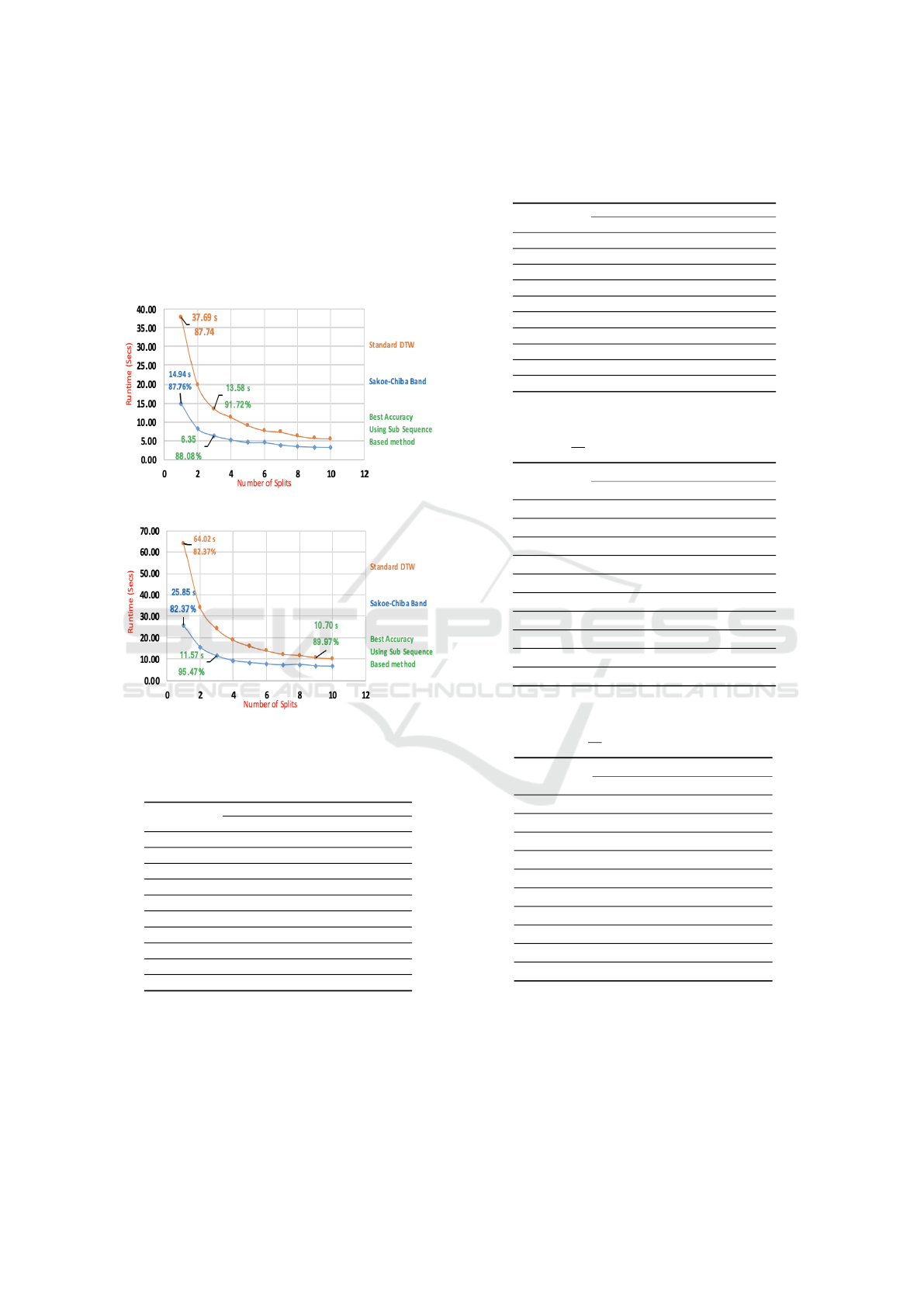
The run time results are presented in Tables 3 to

6. From the tables it can be seen that, as expected,

as s increased the recorded runtime correspondingly

decreased. Figure 7 and 8 show the ﬁxed number of

sub-sequences runtime results, taken from Tables 3

and 4, for two selected data sets, “Lighting2” dataset

and “ShapeletSim” dataset. In the ﬁgures, best re-

sults, using the Sub-Sequence-Based approach, are

highlighted in green. For completeness, best results

without sub-sequencing are also included (s = 1).

The accuracy results are given in Tables 7 and 8.

KDIR 2019 - 11th International Conference on Knowledge Discovery and Information Retrieval

278

From the tables, it can be seen that the accuracy ob-

tained using a ﬁxed number of sub-sequences was bet-

ter than the accuracy obtained using ﬁxed length sub-

sequences. However, there was no single best value

for s. Therefore, it is suggested that the best value of

s should be learnt using a training data set as in the

case of work on learning warping windows (Niennat-

trakul and Ratanamahatana, 2009).

Figure 7: Runtime Results for Lighting2 Dataset.

Figure 8: Runtime Results for ShapeletSim Dataset.

Table 3: Recorded runtime (Secs) using ﬁxed number time

series sub-sequences, the Standard DTW, and a range of val-

ues for s.

Dataset

1 3 5 7 9

GunPoint 8.11 5.03 4.54 4.38 4.26

OliveOil 8.06 3.28 2.44 1.98 1.7

Trace 18.41 7.33 5.57 4.79 4.91

ToeSegment2 23.81 9.06 6.82 6.18 5.29

Car 32.45 11.37 7.49 6.19 5.12

Lightning2 37.69 13.58 9.18 7.35 5.75

ShapeletSim 64.02 24.13 16.00 12.36 10.7

DiatomSizeRed 77.91 30.83 22.10 18.38 16.87

Adiac 156 74.83 65.94 60.87 58.3

HouseTwenty 727 224 133 93 74.3

6.3 Performance Comparison

The performance of the proposed Sub-Sequence-

Based method, in terms of accuracy and the F1 mea-

sure, compared to standard approaches, is considered

in this sub-section. The best results are presented in

Table 4: Recorded runtime (Secs) using ﬁxed number time

series sub-sequences, the Sakoe-Chiba band, and a range of

values for s.

Dataset

1 3 5 7 9

GunPoint 5.51 3.72 4.56 4.30 4.11

OliveOil 4.03 1.98 1.52 1.40 1.25

Trace 8.18 4.65 4.25 3.96 3.78

ToeSegment2 10.1 5.13 4.66 4.31 4.14

Car 13.67 5.5 4.25 3.50 3.20

Lightning2 14.94 6.35 4.63 3.98 3.39

ShapeletSim 25.85 11.57 8.37 7.47 6.79

DiatomSizeRed 34.21 17.11 13.52 13.37 12.21

Adiac 83.58 55.34 52.65 51.93 51.41

HouseTwenty 328.21 84.26 49.94 37.36 29.76

Table 5: Recorded runtime (Secs) using ﬁxed length time

series sub-sequences, the standard DTW, and a range of val-

ues for len (s =

len

Dataset Name

len

10 20 30 40 50

GunPoint 7.26 6.94 6.92 6.74 6.56

OliveOil 1.96 1.90 1.81 1.81 1.77

Trace 7.27 7.19 7.12 6.76 6.58

ToeSegment2 7.90 7.63 7.58 7.52 7.03

Car 5.04 4.72 4.72 4.41 4.25

Lightning2 5.83 5.49 5.48 5.26 4.92

ShapeletSim 13.41 12.31 12.25 11.96 11.71

DiatomSizeRed 24.25 22.33 21.29 21.04 19.72

Adiac 101.00 98.71 98.32 96.55 91.99

HouseTwenty 22.65 20.43 19.47 17.03 16.57

Table 6: Recorded runtime (Secs) using ﬁxed length time

series sub-sequences, the Sakoe-Chiba band, and a range of

values for len (s =

len

Dataset Name

length

10 20 30 40 50

GunPoint 7.75 7.36 6.37 6.28 6.10

OliveOil 2.63 1.85 1.64 1.57 1.56

Trace 6.8 5.93 5.78 5.53 5.47

ToeSegment2 7.11 6.57 6.00 5.87 5.77

Car 4.55 3.82 3.75 3.69 3.62

Lightning2 5.71 4.33 4.16 4.12 4.08

ShapeletSim 11.45 9.81 9.17 9.46 9.05

DiatomSizeRed 20.44 18.48 17.81 16.87 16.54

Adiac 96.06 89.89 85.01 84.77 83.77

HouseTwenty 18.64 13.18 12.92 12.34 12.11

Table 7 and 8, and included the s values that pro-

duced the best results. The ﬁgures in parenthesis are

the standard deviations recorded after averaging over

the ten folds of the TCV. From the table it can be

seen that the performance using the proposed split-

ting method is not adversely affected; in some cases,

the performance improves. Where the performance is

Sub-Sequence-Based Dynamic Time Warping

279

Table 7: Fixed Number: Best accuracy and F1 results, overall best accuracies and F1 values highlighted in bold font.

ID #

Dataset

Benchmark

Standard

DTW

Splitting

Standard

DTW

DTW Using

the S-C Band

` = 10%

Splitting

the S-C Band

`=10%

Acc

(SD)

Acc

(SD)

Acc

(SD)

Acc

(SD)

1 GunPoint

93.97

(0.04)

0.94

(0.05)

4, 7,

8, 10

99.00

(0.02)

0.99

(0.02)

97.47

(0.02)

0.98

(0.03)

100

(0.00)

1.00

(0.00)

2 OliveOil

89.52

(0.15)

0.88

(0.16)

4, 8,

90.95

(0.16)

0.91

(0.16)

98.50

(0.15)

0.89

(0.16)

4, 7, 8,

9, 10

90.95

(0.13)

0.90

(0.14)

3 Trace

99.00

(0.03)

0.99

(0.03)

99.00

(0.03)

0.99

(0.03)

99.00

(0.03)

0.99

(0.03)

98.50

(0.05)

0.99

(0.05)

4 ToeSegment

89.07

(0.09)

00.88

(0.10)

93.33

(0.05)

0.93

(0.05)

92.71

(0.06)

0.92

(0.07)

92.23

(0.04)

0.92

(0.04)

5 Car

80.83

(0.07)

0.80

(0.09)

82.50

(0.07)

0.82

(0.09)

81.67

(0.07)

0.81

(0.08)

83.33

(0.11)

0.82

(0.13)

6 Lighting2

87.74

(0.09)

0.87

(0.08)

91.72

(0.05)

0.91

(0.06)

87.76

(0.08)

0.87

(0.09)

88.08

(0.09)

0.88

(0.10)

7 DiatomSizeReduct

99.36

(0.01)

0.99

(0.01)

6 - 10

100

(0.00)

1.00

(0.00)

99.69

(0.01)

0.99

(0.01)

2 - 10

100

(0.00)

1.00

(0.00)

8 ShapeletSim

82.37

(0.09)

0.81

(0.11)

89.97

(0.06)

0.90

(0.06)

82.37

(0.11)

0.82

(0.11)

95.47

(0.04)

0.96

(0.04)

9 Adiac

64.63

(0.03)

0.62

(0.04)

65.74

(0.03)

0.63

(0.03)

64.63

(0.03)

0.62

(0.04)

65.89

(0.03)

0.63

(0.03)

10 HouseTwenty

95.00

(0.03)

0.95

(0.05)

95.00

(0.03)

0.95

(0.05)

93.08

(0.05)

0.93

(0.05)

93.71

(0.04)

0.93

(0.05)

Table 8: Fixed Length: Best accuracy and F1 results, overall best accuracies and F1 values highlighted in bold font.

Dataset

Name

Benchmark

Standard

DTW

Splitting

Standard

DTW

DTW Using

the S-C Band

` = 10%

Splitting

the S-C Band

` = 10%

Acc

(SD)

Size

Acc

(SD)

Acc

(SD)

Size

Acc

(SD)

1 GunPoint

93.97

(0.04)

0.94

(0.05)

99.47

(0.02)

0.99

(0.02)

97.47

(0.02)

0.98

(0.03)

99.00

(0.03)

0.99

(0.03)

2 Olive Oil

89.52

(0.15)

0.88

(0.16)

10 - 50

90.95

(0.16)

0.91

(0.16)

98.50

(0.15)

0.89

(0.16)

10,

30 - 50

90.95

(0.13)

0.90

(0.14)

3 Trace

99.00

(0.03)

0.99

(0.03)

4, 50

97.50

(0.03)

0.98

(0.04)

99.00

(0.03)

0.99

(0.03)

96.00

(0.06)

0.96

(0.07)

4 Toe Segment

89.07

(0.09)

00.88

(0.10)

92.75

(0.06)

0.92

(0.06)

92.71

(0.06)

0.92

(0.07)

90.46

(0.06)

0.90

(0.07)

5 Car

80.83

(0.07)

0.80

(0.09)

83.33

(0.10)

0.82

(0.11)

81.67

(0.07)

0.81

(0.08)

83.33

(0.09)

0.82

(0.10)

6 Lighting2

87.74

(0.09)

0.87

(0.08)

83.30

(0.06)

0.83

(0.06)

87.76

(0.08)

0.87

(0.09)

84.07

(0.08)

0.88

(0.10)

7 DiatomSize Reduct

99.36

(0.01)

0.99

(0.01)

10 - 50

100

(0.00)

1.00

(0.00)

99.69

(0.01)

0.99

(0.01)

10 - 50

100

(0.00)

1.00

(0.00)

8 ShapeletSim

82.37

(0.09)

0.81

(0.11)

89.97

(0.06)

0.90

(0.06)

82.37

(0.11)

0.82

(0.11)

89.42

(0.08)

0.89

(0.08)

9 Adiac

64.63

(0.03)

0.62

(0.04)

65.51

(0.04)

0.63

(0.04)

64.63

(0.03)

0.62

(0.04)

65.17

(0.06)

0.62

(0.07)

10 HouseTwenty

95.00

(0.03)

0.95

(0.05)

93.71

(0.06)

0.94

(0.06)

93.08

(0.05)

0.93

(0.05)

93.04

(0.05)

0.93

(0.06)

KDIR 2019 - 11th International Conference on Knowledge Discovery and Information Retrieval

280

improved, it is conjectured that this is because the ef-

fect of noise is reduced when using splitting. The re-

sults highlight the issue of selecting the best number

of splits, as noted earlier, there is no single best value

for s. In some cases, there is a range of values for s

that give the same accuracy and F1 score (GunPoint

and OliveOil).

7 CONCLUSION

In this paper, a novel technique (known as Sub-

Sequence-Based DTW) to speed-up runtime of DTW

has been proposed. An analysis of the runtime

complexity and accuracy of DTW using the Sub-

Sequence-Based method was presented. The analy-

sis was conducted with ten time series datasets us-

ing the kNN classiﬁcation technique with k = 1. Dif-

ferent numbers of splits (sub-sequences), deﬁned us-

ing the parameter s were considered. A compari-

son between the Sub-Sequence-Based approach and

Standard DTW and Standard DTW coupled with the

Sakoe-Chiba Band was also presented. The recorded

evaluation results indicated that the DTW runtime us-

ing the Sub-Sequence-Based approach decreases as

the number of splits increased. The effect of s on

accuracy depends on the nature of the data, there-

fore it is suggested that selecting the most appropriate

value for s should be conducted using training data.

It should also be noted that the Sub-Sequence-Based

approach can be applied in any technique founded on

the use of DTW where time series are compared.

REFERENCES

Agrawal, P. and Jayaswal, P. (2019). Diagnosis and classiﬁ-

cations of bearing faults using artiﬁcial neural network

and support vector machine. Journal of The Institution

of Engineers (India): Series C, pages 1–12.

Bagnall, A., Lines, J., Bostrom, A., Large, J., and Keogh,

E. (2017). The great time series classiﬁcation bake

off: a review and experimental evaluation of recent

algorithmic advances. Data Mining and Knowledge

Discovery, 31(3):606–660.

Brunello, A., Marzano, E., Montanari, A., and Sciavicco,

G. (2019). J48ss: A novel decision tree approach for

the handling of sequential and time series data. Com-

puters, 8(1):21.

Byakatonda, J., Parida, B., Kenabatho, P. K., and Moalafhi,

D. (2018). Analysis of rainfall and temperature time

series to detect long-term climatic trends and variabil-

ity over semi-arid botswana. Journal of Earth System

Science, 127(2):25.

Chen, M.-Y. and Chen, B.-T. (2015). A hybrid fuzzy time

series model based on granular computing for stock

price forecasting. Information Sciences, 294:227–

241.

Deng, X., Liu, Q., Deng, Y., and Mahadevan, S. (2016).

An improved method to construct basic probability as-

signment based on the confusion matrix for classiﬁca-

tion problem. Information Sciences, 340:250–261.

Itakura, F. (1975). Minimum prediction residual principle

applied to speech recognition. IEEE Transactions on

Acoustics, Speech, and Signal Processing, 23(1):67–

72.

Niennattrakul, V. and Ratanamahatana, C. A. (2009).

Learning dtw global constraint for time series classiﬁ-

cation. arXiv preprint arXiv:0903.0041.

Rakthanmanon, T., Campana, B., Mueen, A., Batista, G.,

Westover, B., Zhu, Q., Zakaria, J., and Keogh, E.

(2012). Searching and mining trillions of time se-

ries subsequences under dynamic time warping. In

Proceedings of the 18th ACM SIGKDD international

conference on Knowledge discovery and data mining,

pages 262–270. ACM.

Roberts, D. R., Bahn, V., Ciuti, S., Boyce, M. S., Elith, J.,

Guillera-Arroita, G., Hauenstein, S., Lahoz-Monfort,

J. J., Schr

oder, B., Thuiller, W., et al. (2017). Cross-

validation strategies for data with temporal, spatial,

hierarchical, or phylogenetic structure. Ecography,

40(8):913–929.

Sakoe, H. and Chiba, S. (1978). Dynamic programming

algorithm optimization for spoken word recognition.

IEEE transactions on acoustics, speech, and signal

processing, 26(1):43–49.

Silva, D. F. and Batista, G. E. (2016). Speeding up all-

pairwise dynamic time warping matrix calculation. In

Proceedings of the 2016 SIAM International Confer-

ence on Data Mining, pages 837–845. SIAM.

Silva, D. F., Giusti, R., Keogh, E., and Batista, G. E. (2018).

Speeding up similarity search under dynamic time

warping by pruning unpromising alignments. Data

Mining and Knowledge Discovery, 32(4):988–1016.

Singh, A., Thakur, N., and Sharma, A. (2016). A review of

supervised machine learning algorithms. In 2016 3rd

International Conference on Computing for Sustain-

able Global Development (INDIACom), pages 1310–

1315. IEEE.

Tan, C. W., Herrmann, M., Forestier, G., Webb, G. I., and

Petitjean, F. (2018). Efﬁcient search of the best warp-

ing window for dynamic time warping. In Proceed-

ings of the 2018 SIAM International Conference on

Data Mining, pages 225–233. SIAM.

Sub-Sequence-Based Dynamic Time Warping

281