Estimating Configuration Parameters of Pipelines for Accelerating
N-Body Simulations with an FPGA using High-level Synthesis
Tetsu Narumi and Akio Muramatsu
Department of Communication Engineering and Informatics, The University of Electro-Communications,
1-5-1 Chofugaoka, Chofu, Tokyo 182-8585, Japan
Keywords:
FPGA, High-level Synthesis, SDSoC, N-Body Simulation.
Abstract:
In the era of the IoT (Internet of Things) and Edge computing, SoC (System on Chip) with an FPGA (Field
Programmable Gate Array) is a suitable solution for embedded systems because it supports running rich op-
erating systems on general-purpose CPUs, as well as the FPGA’s acceleration for specific computing. One
problem of designing an accelerator on an FPGA is that optimization of the logic for the accelerator is not
automatic and much trial and error is needed before attaining peak performance from the SoC. In this paper
we propose a method to reduce the development time of the accelerator using N-body simulation as a target
application. Based on the hardware resources needed for several pipelines of the accelerator and their perfor-
mance estimation model, we can estimate how many pipelines can be implemented on an SoC. In addition,
the amount of memory each pipeline requires for attaining maximum performance is suggested. Our model
agreed with the actual calculation speed for different constraining conditions.
1 INTRODUCTION
Accelerator architecture, which uses GPUs or
specialized-hardware, is a promising approach to
overcome the increasing demand of huge data pro-
cessing from the Internet. GPUs were initially used
for accelerating scientific simulations, such as N-
body simulations and fluid dynamics (Luebke et al.,
2006). Then, they become a common tool for pro-
cessing Deep Learning operations, such as training
and inference, because highly optimized libraries are
provided from the GPU vendor (Chetlur et al., 2014).
Field Programmable Gate Array (FPGA) is another
solution for data processingwith lowpower consump-
tion, because it can fully optimize specific operations
by reducing the bit length of arithmetic operations.
Even though recent GPUs or CPUs support lower bit-
length arithmetic operations, such as 16-bit floating-
point or 4-bit integer operations, they cannot be used
for arbitrary bit length for each operation.
Another reason that there is a focus on FPGAs is
that they are shipped as an SoC (System on Chip).
In the era of the IoT (Internet of Things), Edge com-
puting is a promising direction because the workloads
on the client side are becoming heavier and the com-
puting power on the server side is not sufficient (Shi
and Dustdar, 2016). Moreover, a reduction of data
from the client side is indispensable to prevent an ex-
plosion of network traffic. An SoC with an FPGA is
a suitable solution because it has a general-purpose
CPU that can run a rich operating system, as well as
an FPGA that can be used as an accelerator for spe-
cific computing (Gomes et al., 2015). The difference
between a pure accelerator with GPUs or FPGAs and
an SoC system is that an SoC system is a compact and
low power system that can be integrated as an Edge
component. We previously proposed an FPGA tablet
that runs Android on the CPU with a specific acceler-
ator for applications configured for the FPGA while
the OS is running (Sato and Narumi, 2015).
One problem of developing an SoC system is de-
signing and optimizing the FPGA. FPGAs are con-
sidered hardware, and designing them with an HDL
(Hardware Description Language) takes far more time
to develop compared with developing such software
for a normal CPU. Recently, High-Level Synthesis
(HLS) has become a useful tool for developing an
FPGA system (Gajski et al., 2012). For example, Sys-
temC (Black et al., 2009) and Vivado HLS (Xilinx,
2019b) are used for such purposes. The last difficulty
is in shortening the design time for establishing the
communication between the CPU and FPGA, which
is not supported by such HLS tools.
SDSoC (Xilinx, 2019a; Kathail et al., 2016) is a
Narumi, T. and Muramatsu, A.
Estimating Configuration Parameters of Pipelines for Accelerating N-Body Simulations with an FPGA using High-level Synthesis.
DOI: 10.5220/0008066500650074
In Proceedings of the 9th International Conference on Pervasive and Embedded Computing and Communication Systems (PECCS 2019), pages 65-74
ISBN: 978-989-758-385-8
Copyright
c
 2019 by SCITEPRESS – Science and Technology Publications, Lda. All rights reserved
65

1 #define EPS2 (0.03f*0.03f)
2 #define MAXN (4096)
3 void force_pipeline(int ioffset, int ni,
4 int nj, float posfi[MAXN][4],
5 float posfj[MAXN][4],
6 float forcef[MAXN][4])
7 {
8 int i, j, k;
9 float dr[3], r_1, dtmp, r2, fi[4];
10
11 for(i=ioffset; i<ioffset + ni; i++){
12 for(k=0; k<4; k++) fi[k]=0.0f;
13 for(j=0; j<nj; j++){
14 #pragma HLS pipeline
15 r2=EPS2;
16 for(k=0; k<3; k++){
17 dr[k]= posfi[i - ioffset][k]
18 - posfj[j][k];
19 r2+= dr[k] * dr[k];
20 }
21 r_1= 1.0f / sqrtf(r2);
22 dtmp= posfj[j][3] * r_1;
23 fi[3]+= dtmp;
24 dtmp*= r_1 * r_1;
25 for(k=0; k<3; k++){
26 fi[k]-= dtmp * dr[k];
27 }
28 }
29 for(k=0; k<4; k++){
30 forcef[i - ioffset][k]=
31 fi[k] * posfi[i - ioffset][3];
32 }
33 }
34 }
Figure 1: Hardware routine for N-body simulation.
tool to shorten the development time when using SoC
with Xilinx FPGAs. It automatically generates com-
munication hardware to bridge the CPU and FPGA,
as well as generating hardware logic on the FPGA, by
just writing with a C-code. By specifying a subrou-
tine to be ported to the hardware, it generates all of
the files needed to operate, such as the OS files and
the bit file to configure the FPGA.
The last difficulty when an accelerator is imple-
mented with the SDSoC is that how to attain max-
imum performance among the various configuration
patterns of the hardware. The effective performance
of the accelerator depends on not only the pure calcu-
lation speed of the hardware pipeline but also the data
transfer speed. Because the SDSoC hides a detailed
mechanism of how the calculation is parallelized as
well as how the CPU and FPGA communicate, much
trial and error is needed when searching for the com-
bination of parameters that achieves the best perfor-
mance. The compilation time of the design of the
FPGA is often very long, and reducing the number
of trials will greatly shorten the development time.
In this paper,we propose a strategy to optimize the
accelerator performance by estimating it beforehand
using N-body simulation as an example. In section 2,
related works on designing accelerators with FPGAs
are described. In section 3, the system architecture
of this work is shown. The performance result and
resource usage are summarized in section 4, and its
estimation is explained in section 5. Finally, section 6
summarizes the paper.
1 void calculate_force(int N, double pos[][4],
2 double force[][4])
3 {
4 float posi[MAXN][4], posj[MAXN][4];
5 float forcef[MAXN][4];
6 int i, k;
7 for(i=0; i<N; i++) for(k=0; k<4; k++){
8 posi[i][k] = (float) pos[i][k];
9 posj[i][k] = (float) pos[i][k];
10 }
11 force_pipeline(0, N, N, posf, posf, forcef);
12 for(i=0; i<N; i++) for(k=0; k<4; k++){
13 force[i][k] = (double) forcef[i][k];
14 }
15 }
Figure 2: Non-parallelized parent routine.
2 RELATED WORK
FPGAs are used to accelerate many applications, such
as encoding for wireless communication (El Adawy
et al., 2017), error correction with a low density par-
ity check (Roh et al., 2016), image processing for 4K
video streams (Kowalczyk et al., 2018), convolutional
and recurrent neural networks (Zeng et al., 2018),
the Finite Difference Time Domain (FDTD) method
(Waidyasooriya et al., 2017), and N-body simulations
(Peng et al., 2016; Del Sozzo et al., 2017; Ukawa and
Narumi, 2015; K&F, 2015).
N-body simulation is an applications that allows
the FPGA to successfully compete with other archi-
tectures, such as GPU. Peng et al. developed a sys-
tem with a Zynq SoC to accelerate an N-body Mod-
ified Newtonian Dynamics (MOND) simulation, and
achieved 10 times better performance per watt com-
pared with an Nvidia K80 GPU (Peng et al., 2016).
GRAPE-9 (K&F, 2015) achieved 16 Tflops of perfor-
mance with only 300W in 2015, while a K20 GPU
could reach only 1/3 of that with similar power con-
sumption at that time. In these implementations, the
pipeline is carefully optimized with much effort, such
as using a lower bit-length of arithmetic units. How-
ever, in this paper, we use only a simple C-code to
develop the pipeline, and concentrate on the proposed
strategy to parallelize the pipeline without much ef-
fort.
The key technology is SDSoC (Xilinx, 2019a)
from Xilinx, which is a kind of High Level Synthe-
sis (HLS) tool. Unlike SystemC or Vivado HLS,
SDSoC automatically generates communication hard-
ware as well as the accelerator itself. Rettkowski et
al. achieved 10 times the acceleration of the His-
togram of Oriented Gradients (HOG) algorithm com-
pared with the ARM processor in the SoC with a
Zynq device (Rettkowski et al., 2017). A Convolu-
tional Neural Network (CNN) and a Recurrent Neu-
ral Network (RNN) were accelerated on Zynq MP-
SoC device, and achieved several times of acceler-
ation compared with previous implementation with
PECCS 2019 - 9th International Conference on Pervasive and Embedded Computing and Communication Systems
66

1 void calculate_force(int N, double pos[][4],
2 double force[][4])
3 {
4 float posi[2][MAXN/2][4], posj[MAXN][4];
5 float forcef[2][MAXN/2][4];
6 int i, k;
7 for(i=0; i<N; i++) for(k=0; k<4; k++){
8 posi[i*2/N][i % N][k] = (float) pos[i][k];
9 posj[i][k] = (float) pos[i][k];
10 }
11 #pragma SDS async(1)
12 force_pipeline(0 ,N/2, N, posfi[0],
13 posfj, forcef[0]);
14 #pragma SDS async(2)
15 force_pipeline2(N/2, N/2, N, posfi[1],
16 posfj, forcef[1]);
17 #pragma SDS wait(1)
18 #pragma SDS wait(2)
19 for(i=0; i<N; i++) for(k=0; k<4; k++){
20 force[i][k] =
21 (double) forcef[i*2/N][i % N][k];
22 }
23 }
Figure 3: Parallelized parent routine.
FPGAs (Zeng et al., 2018). Several filters for 4K
video streaming were also accelerated by SDSoC on a
Zynq MPSoC device (Kowalczyk et al., 2018). They
discussed the merits and drawbacks of using SDSoC
compared with Vivado HLS or the xfOpenCV library.
There are other methods for writing an accelerator
code, including the data transfer portion from a high
level language, such as OpenCL (Khronos,2019). For
example, Neural network and FDTD calculations are
implemented with FPGAs (Luo et al., 2018; Waidya-
sooriya et al., 2017). Though OpenCL can support
many platforms including CPUs and GPUs, we need
to modify the code using specific APIs. However,SD-
SoC requires no modification of the software to use
FPGAs.
Making a performance model is a reasonable
approach to optimizing the hardware accelerator.
Mousouliotis et al. accelerated convolutional neural
networks using SDSoC on Zynq SoC (Mousouliotis
and Petrou, 2019). They modeled such elements as
pipeline depth and function/loop overheads, and they
were consistent in resourcing usage from the vendor
tool. However, their model did not combine hardware
resources and performance to attain a simple answer
for optimized parameters. Zeng et al. also showed
the performance model for neural network accelera-
tor with SDSoC (Zeng et al., 2018), but they just de-
scribed the calculation cost. However, our strategy
directly describes which parameters should be used
to achieve the maximum performance for a specified
condition.
3 SYSTEM ARCHITECTURE
In this section the hardware and software of the sys-
tem is described.
Table 1: Specifications of an Ultra96 board.
Element Description
SoC Xilinx Zynq UltraScale+
MPSoC ZU3EG
RAM 2 GB (512M x32) LPDDR4
Wireless 802.11b/g/n Wi-Fi, Bluetooth 4.2
USB 1x USB 3.0 (up)
2x USB 3.0, 1x USB 2.0 (down)
Display Mini DisplayPort
Power Source 8V∼18V@3A
OS Support Linux
Size 85mm × 54mm
3.1 Hardware Platform
For the SoC platform with an FPGA, we used an Ul-
tra96 board (Avnet, 2019), which houses a Zynq MP-
SoC device. Table 1 shows the specifications. The
SoC contains a quad-core ARM Coretex-A53 proces-
sor operated at 1.5 GHz, a dual-core Cortex-R5 pro-
cessor, a Mali-400 MP2 GPU as well as FPGA func-
tions. However, the most attractive point is its small
size, comparable to a credit card. It is suitable for
Edge IoT devices because it can run the latest OS and
many IO ports are supported. The size of the logic
that fits into the FPGA is not so large compared with
other MPSoC devices, and devices that are 7 times
larger are available on the market. However the op-
timization strategy proposed in this paper would be
more useful for a larger device; larger devices need a
longer compilation time and good estimation methods
are more useful than small devices.
3.2 Software for Parallel Processing of
Pipelines
Figure 1 shows the subroutine to calculate gravity be-
tween particles. Only this routine is converted to the
hardware by SDSoC tool because other calculations
are not so compute intensive. Note that there are
i -
and j -loops (see lines 11 and 13 in Figure 1). Vari-
ables (
posi, posj ) to store particle positions and
calculated forces ( forcef ) are allocated with a fixed
size because SDSoC requests it when a simple com-
munication method is used.
Figure 2 shows a non-parallelized parent routine.
The calculation cost of
calculate force is O(N
2
),
where N is the number of particles. Note that con-
version from
double to float is performed to call
force pipeline , and the results are also converted
back (see lines 8, 9 and 13 in Figure 2). Such con-
version takes some time with a low power CPU in the
SoC.
To attain the highest performance with SDSoC,
three techniques are used.
Estimating Configuration Parameters of Pipelines for Accelerating N-Body Simulations with an FPGA using High-level Synthesis
67

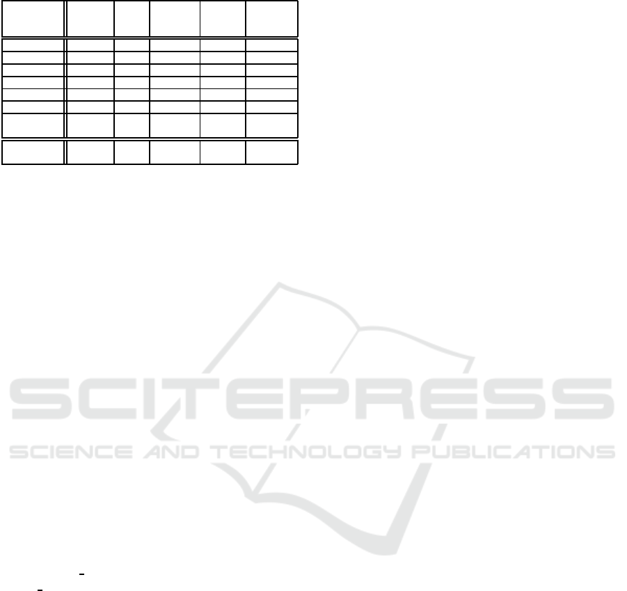
Table 2: Resources for different number of pipelines
(p
unroll
).
Number of Compile
pipelines BRAM DSP FF LUT time
(p
unroll
) (min)
1 170 10 29,094 17,720 23
2 170 20 31,547 19,509 22
4 170 40 36,339 22,530 25
8 170 77 46,485 29,651 28
16 170 151 67,780 44,503 41
25 170 235 88,491 56,522 112
26 - - - - 348
(fail)
Max
Resource 432 360 141,120 70,560
3.2.1 Create a Pipeline
Adding a “ #pragma HLS pipeline ” line (see line 14
in Figure 1) will automatically make a pipeline. The
number of clocks required for getting one result (ini-
tiation interval) is not specified, and it is estimated as
5 in this system based on section 5.1.
3.2.2 Parallel Processing in a Pipeline
Manual loop-unrolling was performed to calculate a
different
i of the for loop in line 11 of Figure 1. We
used a manual one because automatic loop-unrolling
with “
#pragma HLS unroll ” was not successful.
3.2.3 Parallelizing the Whole Pipeline
By duplicating the pipeline and executing both
pipelines simultaneously, further acceleration can be
done. Figure 3 shows a dual pipeline case. First,
the dimensions of
posi and forcef are increased
without increasing the total size of the array. The
particle position ( posi ) is divided into two groups,
and the result (
forcef ) is divided into two ar-
rays. force pipeline2 is the same program as
force pipeline . However, different name is needed
for conversions to different instances in the FPGA
by SDSoC. By using
#pragma SDS async and wait ,
two pipelines are executed simultaneously.
3.2.4 Further Optimization
Further optimization might be possible, but we did not
try other ones because the main object was not opti-
mization of a pipeline itself. For example the follow-
ing methodswould be possible: reduction of initiation
interval, loop-unrolling for the j-loop to reduce the
loop count, reduction of the bit-length of arithmetic
operation, or interpolation for calculating division or
square root (K&F, 2015).
4 PERFORMANCE RESULT AND
RESOURCE USAGE
In this section, several results of calculation speed are
shown as well as how much logic and RAM are used
for the pipeline.
4.1 Parallelization in a Pipeline
Table 2 shows how many resources in the FPGA are
used for the system, which is described in section
3.2.2. The number of pipelines generated by un-
rolling the subroutine is called p
unroll
in this paper.
The size of the local memory,
MAXN in Figure 1, is
fixed to 4096, which is the maximum when compiled
with SDSoC. BRAM means “Block RAM”, which is
used as local memory. DSP is a specialized arithmetic
logic for such functions as addition and multiplica-
tion. FF means Flip-Flops, and LUT means Look-
Up Table for logical operations. “(fail)” means that
the compilation failed to generate 26 pipelines in this
case. The last row shows the maximum number of
resources of the target device.
As shown in the last column of Table 2, the com-
pilation time of SDSoC increases as the number of
pipelines increases. Especially, when it reaches its
limit, the compilation time increases dramatically.
This is the reason that estimating configuration pa-
rameters is important for FPGA development. Among
BRAM, DSP, FF and LUT, LUT is the most restrictive
resource in this case.
Figure 4 shows the calculation speed in Gflops
by changing the number, N, of particles for differ-
ent numbers of pipelines, p
unroll
. Here we assumed
38 floating point operations per pairwise interaction.
Parallel efficiency is 0.92 when p
unroll
= 25 for N =
8192. This number means the speed of 25 pipelines
is 25× 0.92 times faster than that of a single pipeline,
which is sufficient.
4.2 Parallelization of the Whole Pipeline
Table 3 shows how many resources are used for the
system described in section 3.2.3. The number of
pipelines attained by parallelizing the whole pipeline
is called p
dma
because a DMA engine is generated for
each pipeline. The SDSoC automatically generates a
data motion network, which communicates between
the CPU and FPGA. In this paper we do not specify
which data motion network should be used, and the
SDSoC automatically chooses the best one.
The required resources in this section is much
higher than that presented in the previous section.
Only seven pipelines can be implemented instead
PECCS 2019 - 9th International Conference on Pervasive and Embedded Computing and Communication Systems
68

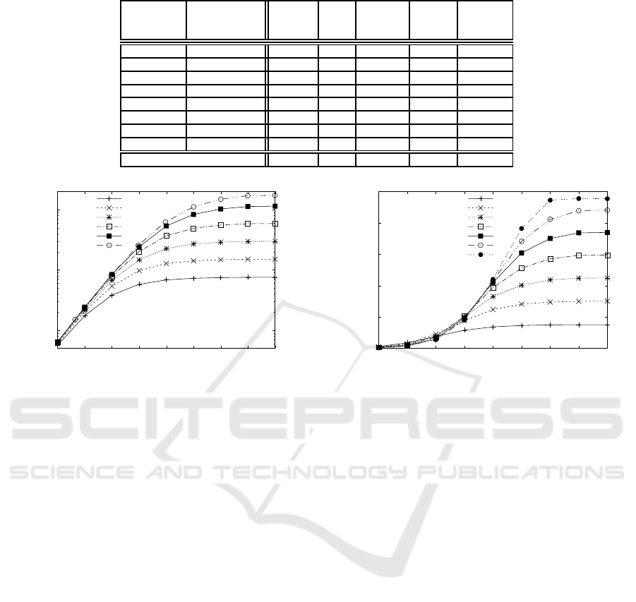
Table 3: Resources for different numbers of pipelines (p
dma
).
Number of Size of Compile
pipelines local memory BRAM DSP FF LUT time
(p
dma
) (N
local
) (min)
1 4,096 170 10 29,094 17,720 23
2 4,096 226 20 42,868 26,155 35
3 4,096 297 30 51,600 32,527 48
4 4,096 304 40 60,249 38,817 45
5 4,096 367 50 71,236 46,411 62
6 4,096 430 60 82,231 54,008 72
7 2,048 325 70 93,134 61,481 103
8 2,048 - - - 74,565 72 (fail)
Max resource 432 360 141,120 70,560
0.1
1
10
32 64 128 256 512 1024 2048 4096 8192
Calculation Speed (Gflops)
Number of Particles
p= 1
p= 2
p= 4
p= 8
p=16
p=25
Figure 4: Calculation speed with different numbers of
p
unroll
.
of 25 pipelines. The bottleneck of the resources is
BRAM, as shown in Table 3. Because the number of
BRAMs exceeds the limit when seven pipelines are
used, the N
local
value is reduced from 4096 to 2048.
Here, N
local
is the same as
MAXN in Figure 1. The sum
of the data-transfer size of
posi and forcef is fixed
to MAXN ×4 and that of posj is proportional to p
dma
,
as shown in Figure 3. Note that though the size of
posj seems to be fixed in the C-code level, the actual
hardware needs a different buffer for each pipeline to
receive data in
posj .
Figure 5 shows the calculation speed. Compared
with Figure 4, the highest speed is much lower. In
addition, the line of p
dma
= 7 becomes horizontal in
a larger number of particles. This is because N
local
is
smaller than other cases, which causes low efficiency
because of communication overhead. The parallel ef-
ficiency is 0.90 when p
dma
= 7 for N = 8192, which
is already lower than the 0.92 of the p
unroll
= 25 case.
4.3 Combining Both Parallelizations
Table 4 shows the hardware resources needed for the
same number of parallelisms but different combina-
tions of parallelization methods. Here we call the
0
1
2
3
4
5
32 64 128 256 512 1024 2048 4096 8192
Calculation Speed (Gflops)
Number of Particles
p=1, Nlocal=4k
p=2, Nlocal=4k
p=3, Nlocal=4k
p=4, Nlocal=4k
p=5, Nlocal=4k
p=6, Nlocal=4k
p=7, Nlocal=2k
Figure 5: Calculation speed with different numbers of p
dma
.
total number of pipelines p:
p = p
dma
p
unroll
. (1)
As seen in Table 4, using p
unroll
first is always
better than using a p
dma
parallelism. For example,
when p = 16, the lowest BRAM usage comes from
the combination {p
unroll
=16, p
dam
=1}. DSP, FF, LUT
and compilation time are also the lowest for the same
combination.
Figure 6 compares the calculation speed. The
peak speed has no difference when p is the same, but
a larger p
dma
causes more overhead around N = 512.
Therefore, using lower p
dma
is also better from the
point of view of performance.
For obtaining maximum performance from this
SoC, we have no reason to use the p
dma
parallelism.
However, to use the p
unroll
parallelism, one needs
manual unrolling, as described in section 3.2.2, which
increases the development cost for the software side,
especially when we have to try with different numbers
of parallelism. In addition, the communicationperfor-
mance might be better in different platforms because
using independent DMA engines might increase the
data transfer. Therefore, in the rest of this paper, we
concentrate on using the p
dma
parallelism because the
optimization strategy is not straight forward.
Estimating Configuration Parameters of Pipelines for Accelerating N-Body Simulations with an FPGA using High-level Synthesis
69

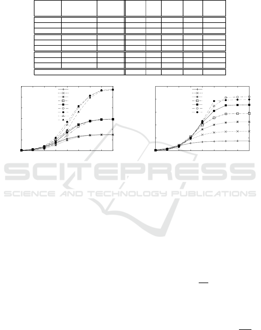
Table 4: Resources according to parallelism.
Number of Number of Number of Compile
pipelines DMA instances unrolling BRAM DSP FF LUT time
(p) (p
dma
) (p
unroll
) (min)
4 1 4 170 40 36,339 22,530 25
4 2 2 226 40 47,766 29,726 31
4 4 1 304 40 60,249 38,817 45
8 1 8 170 77 46,485 29,651 28
8 2 4 226 80 57,328 35,786 32
8 4 2 304 80 70,029 46,007 30
16 1 16 170 151 67,780 44,503 41
16 2 8 226 154 77,594 50,030 44
16 4 4 304 160 89,133 58,024 65
Max resource 432 360 141,120 70,560
0
2
4
6
8
10
12
32 64 128 256 512 1024 2048 4096 8192
Calculation Speed (Gflops)
Number of Particles
p= 4(d1, u4)
p= 4(d2, u2)
p= 4(d4, u1)
p= 8(d1, u8)
p= 8(d2, u4)
p= 8(d4, u2)
p=16(d1,u16)
p=16(d2, u8)
p=16(d4, u4)
Figure 6: Calculation speed for the same number of
pipelines.
4.4 Lower Resources of BRAM
Table 5 and Figure 7 show the case when the maxi-
mum resources of BRAM are limited to 300 instead
of 432. This situation is when BRAM is used for an-
other purpose in the design and we can use only 300
of the 432 BRAMs for the pipeline. Only the p
dma
parallelism is used, as in Table 3 and Figure 5.
The difference caused by the new limitation is that
N
local
needs to be decreased to reduce the consump-
tion of the BRAM. The number of pipelines is the
same because LUT becomes the bottleneck subse-
quent to BRAM. The large difference in calculation
speed between Figures 5 and 7 is because p
dma
=
7 causes a lower speed compared with the smaller
p
dma
= 6. This did not happen in Figure 5. This is
because a lower N
local
causes more overhead in the
communication between the CPU and FPGA. In the
following sections we analyze this further.
5 PERFORMANCE ESTIMATION
In this section, we first show the performance model.
Then, we make a model for resource estimation. Fi-
0
1
2
3
4
5
32 64 128 256 512 1024 2048 4096 8192
Calculation Speed (Gflops)
Number of Particles
p=1, Nlocal=4k
p=2, Nlocal=4k
p=3, Nlocal=4k
p=4, Nlocal=2k
p=5, Nlocal=2k
p=6, Nlocal=2k
p=7, Nlocal=1k
Figure 7: Calculation speed when a lower number of
BRAMs is used.
nally, we show graphs to choose the best parameter
among many possibilities.
5.1 Performance Model
The time needed for one step for an N-body simula-
tion cab be expressed as:
T = T
fpga
+ T
comm
, (2)
where T
fpga
is the calculation time in the hardware
pipeline in the FPGA, and T
comm
is the communica-
tion time between the CPU and the pipeline.
T
fpga
is expressed as:
T
fpga
=
t
fpga
p
N
2
, (3)
where N is the number of particles, p is the number
of pipelines, and t
fpga
is the time for a pairwise force
calculation between particles with a single pipeline.
T
comm
can be expressed as:
T
comm
= {t
band
N
local
(p
dma
+ 2) +t
lat
p
dma
}⌈
N
N
local
⌉
2
,
(4)
where t
band
is the communication time needed to
transfer data for a particle, which is 16 bytes because
PECCS 2019 - 9th International Conference on Pervasive and Embedded Computing and Communication Systems
70

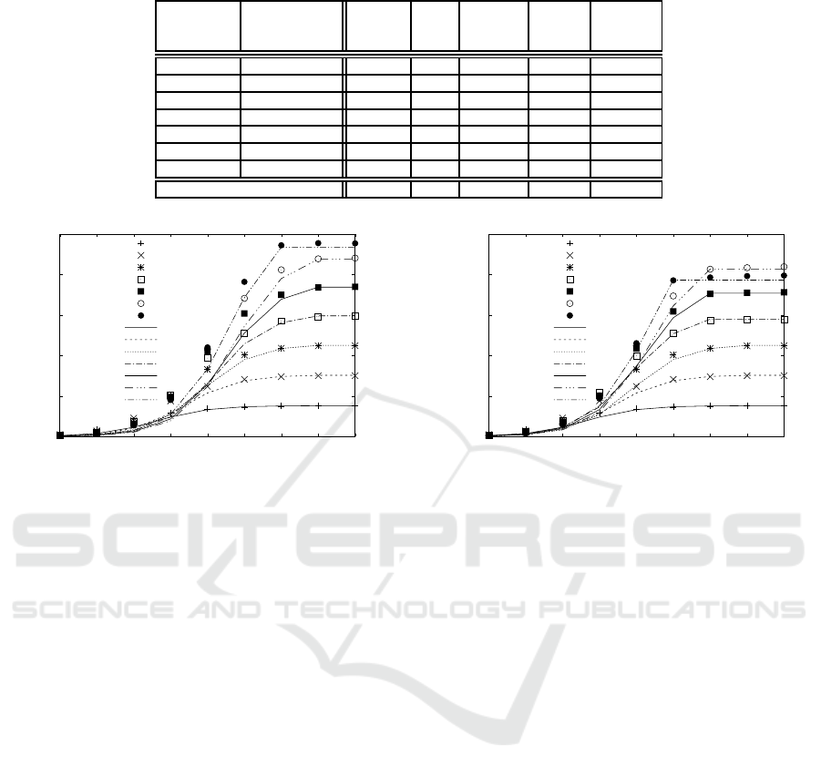
Table 5: Resources used when the maximum number of BRAM is reduced.
Number of Size of Compile
pipelines local memory BRAM DSP FF LUT time
(p
dma
) (N
local
) (min)
1 4,096 170 10 29,094 17,720 23
2 4,096 226 20 42,868 26,155 35
3 4,096 297 30 51,600 32,527 48
4 2,048 208 40 60,197 38,716 59
5 2,048 247 50 71,171 46,305 66
6 2,048 286 60 82,153 53,866 58
7 1,024 241 70 93,029 61,345 129
Max resource 300 360 141,120 70,560
0
1
2
3
4
5
32 64 128 256 512 1024 2048 4096 8192
Calculation Speed (Gflops)
Number of Particles
p=1
p=2
p=3
p=4
p=5
p=6
p=7
p=1 est
p=2 est
p=3 est
p=4 est
p=5 est
p=6 est
p=7 est
Figure 8: Estimated calculation speed.
four
float variables are used. t
lat
is the setup time
needed to initiate the communication. ⌈x⌉ represents
an integer larger or equal to x. When N > N
local
,
we need to replace the contents of particle memory,
which causes the overhead of communication.
Table 6 summarizes the parameters for perfor-
mance estimation. To determine t
fpga
, the difference
of T between {p=1, N=4096, N
local
=4096} and {p=1,
N=2048, N
local
=4096} is used because only the T
fpga
part is different. For t
lat
, the difference of T be-
tween {p
dma
=1, p
unroll
=1, N=256, N
local
=4096} and
{p
dma
=4, p
unroll
=1, N=512, N
local
=2048} is used be-
cause only the latency part is different. For t
band
, T of
{p
dma
=7, p
unroll
=1, N=1024, N
local
=1024} is used.
t
fpga
= 5.0 × 10
−8
means the calculation of the
force on a particle is executed every 50 ns, which cor-
respond to 20 MHz. Because the clock frequency of
the pipeline is fixed to 100 MHz in SDSoC configu-
ration in this paper, the initiation interval is 5 instead
of 1. Further optimization of the interval is out of the
scope of this paper as described in section 3.2.4.
t
band
= 1.4× 10
−7
corresponds to 114 Mbyte/s of
data transfer speed, which is far lower than the peak
band width, 4 Gbyte/s, of the DDR4 DRAM on the
Ultra96 board. This is because t
band
includes opera-
tions other than pure data transfer, such as conversion
from
double to float and copy to a temporary buffer
for communication with the FPGA.
0
1
2
3
4
5
32 64 128 256 512 1024 2048 4096 8192
Calculation Speed (Gflops)
Number of Particles
p=1
p=2
p=3
p=4
p=5
p=6
p=7
p=1 est
p=2 est
p=3 est
p=4 est
p=5 est
p=6 est
p=7 est
Figure 9: Estimated calculation speed when BRAM is re-
duced.
Figures 8 and 9 show the estimated performance
in lines, while measured results are still shown as
points. As can be seen, the estimation is roughly con-
sistent to the measurement except for middle range
of the number of particles (128 ≤ N ≤ 512). Even
though the quantitative value for the middle range of
the number of particles is different from the actual
data, the order of estimated times are consistent with
the data, i.e., a larger p
dma
causes lower performance.
5.2 Resource Estimation
In this section, resource parameters for BRAM and
LUT are considered because DSP and FF do not be-
come the bottleneck in our case. In this estimate,
only the parallelization of the whole pipeline (Section
4.2) is assumed because parallelization in the pipeline
(Section 4.1) is too simple for estimation.
The total number of BRAMs, B
total
, can be esti-
mated as:
B
total
= (B
mem
N
local
+ B
dma
)p
dma
+ B
other
, (5)
where B
dma
is the number of BRAM blocks for data
transfer. B
mem
is the number of BRAMs for storing
particle positions and forces, and B
other
is the number
of BRAMs required for other than the pipeline itself.
Total number of LUT units, L
total
, is estimated as:
L
total
= L
pipe
p
dma
+ L
other
, (6)
Estimating Configuration Parameters of Pipelines for Accelerating N-Body Simulations with an FPGA using High-level Synthesis
71

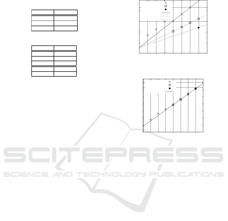
Table 6: Configuration parameters for performance estima-
tion.
Parameter Value
t
fpga
5.0× 10
−8
t
band
1.4× 10
−7
t
lat
2.2× 10
−4
Table 7: Configuration parameters for resource estimation.
Parameter Value
B
mem
12 / 1,024
B
dma
15
B
other
52
L
pipe
7,600
L
other
8,300
where L
pipe
is the number of LUT units for a pipeline
as well as the DMA controller, and L
other
is LUT for
other type of logic.
Table 7 summarizes the parameters for hardware
resources. To determine B
mem
, the difference of
BRAM between {p
dma
=4, p
unroll
=1, N
local
=4096} and
{p
dma
=4, p
unroll
=1, N
local
=2048} are used in Tables
3 and 5. Similarly, to determine B
dma
, the differ-
ence between {p
dma
=4, p
unroll
=1, N
local
=4096} and
{p
dma
=5, p
unroll
=1, N
local
=4096} are used in Table 3.
Then B
other
is calculated from the data of {p
dma
=4,
p
unroll
=1, N
local
=4096}.
To determine L
pipe
, the difference of LUTs be-
tween {p
dma
=4, p
unroll
=1, N
local
=2048} and {p
dma
=5,
p
unroll
=1, N
local
=2048} are used in Table 5. Then
L
other
is calculated from the case of {p
dma
=4,
p
unroll
=1, N
local
=2048}.
Figures 10 and 11 show the estimated values in
lines against actual values in points. As for BRAM,
two limits are shown as horizontal lines. Estimated
lines fit perfectly for large p
dma
, while the lines es-
timate much lower values than the actual usage for
small p
dma
. The reason is that the optimization of re-
source usage is not performed when resources are not
so severely restricted (sparse layout could be done).
As for LUT, the two horizontal lines indicate the
maximum and 90% of the maximum LUTs. Using
100% of the LUT is difficult with FPGA because the
layout of the logic becomes too difficult. In this esti-
mate, we choose 90% as the practical limit. The dif-
ference, depending on N
local
, is very small and we did
not include such a parameter for LUT, unlike what
we did for BRAM. For small p
dma
, the actual number
of LUTs is larger than the estimated number, which
arises from the same reason that optimization of log-
ics is not needed so much at the compile and layout
stage.
0
100
200
300
400
500
0 1 2 3 4 5 6 7 8
300
432
Number of BRAM blocks (B
total
)
p
dma
Nlocal=4k
Nlocal=2k
Nlocal=1k
4k est
2k est
1k est
Figure 10: Estimated number of BRAMs (B
total
).
0
10000
20000
30000
40000
50000
60000
70000
0 1 2 3 4 5 6 7 8
63504
70560
Number of LUTs (L
total
)
p
dma
Nlocal=4k
Nlocal=2k
Nlocal=1k
Est
Figure 11: Estimated number of LUTs (L
total
).
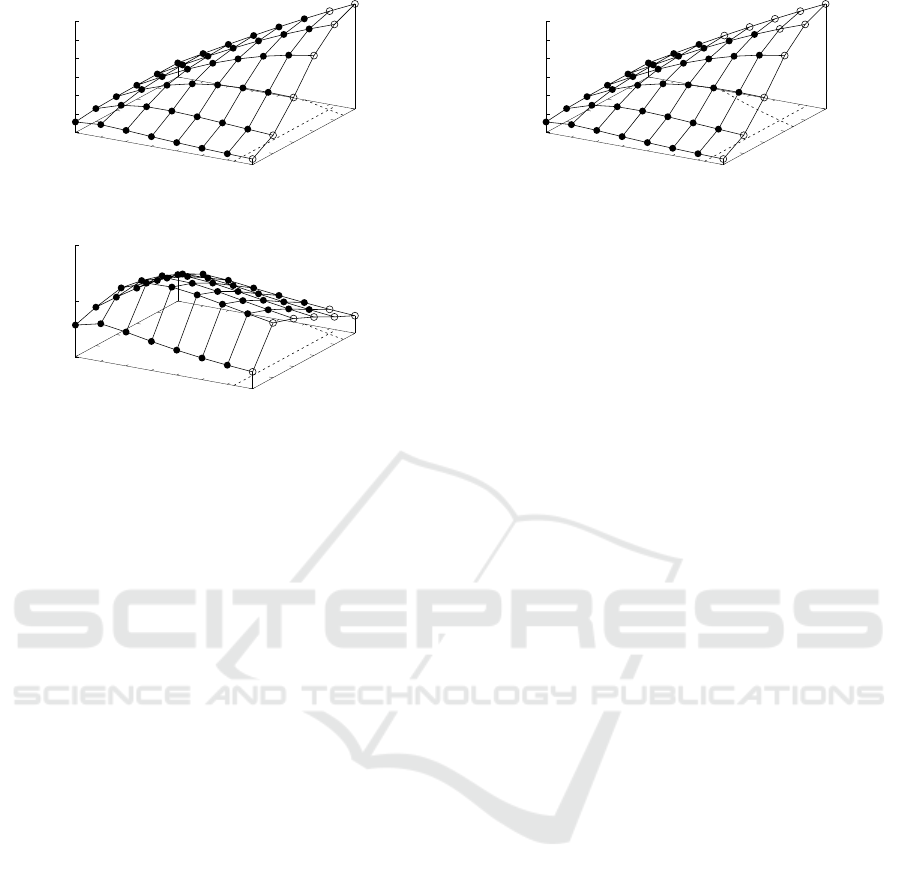
5.3 Estimation of the Best
Configuration Parameters
In this section, we finally estimate the configuration
parameters, i.e., p
dma
and N
local
in our case. We
assume three cases: A) N=8192 and B
max
=432, B)
N=256 and B
max
=432, and C) N=8192 and B
max
=300.
Here B
max
is the maximum number of BRAMs al-
lowed for the accelerator.
Figure 12 shows the estimated parameters for case
A). The two dotted lines at the base indicate the
boundaryof limitations calculated by Eqs. (5) and (6).
The filled-circle indicates that the values are within
the range of the limitations, while the open circle in-
dicates values that are out of range. p
dma
=8 is al-
ways out of range, and only {p
dma
=7, N
local
=4096}
is also out of range for p
dma
=7. The highest per-
formance is estimated to be achieved when {p
dma
=7,
N
local
=2048}, which is consistent with Figure 5.
Figure 13 is for case B), in which the number of
particles are small. Small N needs a small N
local
for
high efficiency, as well as a small number of pipelines.
The small N
local
is required for reducing the data size
for transfer, and the small p
dma
is for low latency
to start the DMAs. The highest performance is es-
timated to be achieved when {p
dma
=4, N
local
=256}
({p
dma
=3, N
local
=256} is very similar).
PECCS 2019 - 9th International Conference on Pervasive and Embedded Computing and Communication Systems
72

1
2
3
4
5
6
7
8
128
256
512
1024
2048
4096
0
1
2
3
4
5
6
p
dma
N
local
Calculation Speed (Gflops)
Figure 12: Possible parameters for case A).
1
2
3
4
5
6
7
8
128
256
512
1024
2048
4096
0
1
2
p
dma
N
local
Calculation Speed (Gflops)
Figure 13: Possible parameters for case B).
Figure 14 is for case C), where the maximum
number of BRAMs is reduced. Open circles are in-
creased compared with the other cases. These are
consistent with the actual possible parameters in Ta-
ble 5. The highest performance is suggested when
{p
dma
=6, N
local
=2048}, which is also consistent with
Figure 7.
6 CONCLUSION
In this paper, we proposed an optimization strategy to
determine the configurationparameters of pipelines to
accelerate N-body simulations. The method is sum-
marized into following three steps.
First, we measure the consumed resources for im-
plementing a middle range of a number of pipelines.
A low number of pipelines is not good for estima-
tion because the logics are not sufficiently optimized.
However, a full number of pipelines is not suitable ei-
ther because of the long compilation time.
Second, both performance and resource models
are generated based on the measurement. By chang-
ing only one parameter among several, we can know
the coefficient depending on the parameter. For better
fitting, data from the middle range of the number of
pipelines should be used, as pointed out above.
Third, make a graph for searching the best com-
bination of parameters by integrating all the models
and constraints into a single view. Once the model is
generated, we can easily change the constraints: the
maximum number of BRAM units (B
max
), maximum
number of LUT units, and the number of particles (N),
in our case. Then, the best combination of the num-
1
2
3
4
5
6
7
8
128
256
512
1024
2048
4096
0
1
2
3
4
5
6
p
dma
N
local
Calculation Speed (Gflops)
Figure 14: Possible parameters for case C).
ber of pipelines (p
dma
) and the size of the local mem-
ory (N
local
) are estimated. The estimation reasonably
agreed with the measurements.
With our strategy, we can reduce the development
time for optimizing the accelerator great deal because
the effective calculation speed is well estimated even
for unknown combinations of parameters. As shown
in Tables 3 and 5, the compilation time for a mid-
dle range of the number of pipelines is roughly half
the compilation time needed for a full number of
pipelines. Moreover, when the compilation fails be-
cause of a bad estimate, we need much more time to
search the best one. A good estimate can avoid such
a waste of time. Improvements should be made to
reduce the disagreement for the middle range of the
number of particles.
The most important part of our strategy is the per-
formance model. Even with a simple N-body sim-
ulation, there are several methods to parallelize the
calculation. The overhead greatly depends on how it
is parallelized, especially when the resources are lim-
ited. Therefore, a good performance model should
be carefully investigated for Edge devices. When the
strategy is used for Deep Neural Network (DNN) ap-
plications, it would be more challenging to make per-
formance models because they have more parameters,
such as the depth of layers, the size of each layer, and
the size of a convolution kernels. However, a similar
strategy to that proposed in this paper would work for
a quick estimation of the configuration parameters.
Future research should include applying this strat-
egy for larger devices as well as different architec-
tures. Several kinds of accelerators need to be inves-
tigated for further application of our method. Also,
fully optimizing the pipeline for N-body simulation
to compare previous research is another direction of
the next study.
ACKNOWLEDGMENTS
This work was partially supported by JSPS KAK-
ENHI (Grant Number 17K00267).
Estimating Configuration Parameters of Pipelines for Accelerating N-Body Simulations with an FPGA using High-level Synthesis
73

REFERENCES
Avnet (2019). Ultra96 - 96boards. https://www.96boards.
org/product/ultra96/. (Accessed on 04/29/2019).
Black, D. C., Donovan, J., Bunton, B., and Keist, A. (2009).
SystemC: From the ground up, volume 71. Springer
Science & Business Media.
Chetlur, S., Woolley, C., Vandermersch, P., Cohen, J., Tran,
J., Catanzaro, B., and Shelhamer, E. (2014). cudnn:
Efficient primitives for deep learning. arXiv preprint
arXiv:1410.0759.
Del Sozzo, E., Di Tucci, L., and Santambrogio, M. D.
(2017). A highly scalable and efficient parallel design
of n-body simulation on fpga. In 2017 IEEE Interna-
tional Parallel and DistributedProcessing Symposium
Workshops (IPDPSW), pages 241–246. IEEE.
El Adawy, M., Kamaleldin, A., Mostafa, H., and Said, S.
(2017). Performance evaluation of turbo encoder im-
plementation on a heterogeneous fpga-cpu platform
using sdsoc. In 2017 Intl Conf on Advanced Control
Circuits Systems (ACCS) Systems & 2017 Intl Conf on
New Paradigms in Electronics & Information Technol-
ogy (PEIT), pages 286–290. IEEE.
Gajski, D. D., Dutt, N. D., Wu, A. C., and Lin, S. Y. (2012).
High—Level Synthesis: Introduction to Chip and Sys-
tem Design. Springer Science & Business Media.
Gomes, T., Pinto, S., Tavares, A., and Cabral, J. (2015).
Towards an fpga-based edge device for the internet of
things. In 2015 IEEE 20th Conference on Emerging
Technologies & Factory Automation (ETFA), pages 1–
4. IEEE.
Kathail, V., Hwang, J., Sun, W., Chobe, Y., Shui, T., and
Carrillo, J. (2016). Sdsoc: A higher-level program-
ming environment for zynq soc and ultrascale+ mp-
soc. In Proceedings of the 2016 ACM/SIGDA Interna-
tional Symposium on Field-Programmable Gate Ar-
rays, pages 4–4. ACM.
K&F (2015). K & f computing research. http://www.kfcr.jp/
grape9.html. (Accessed on 04/29/2019).
Khronos (2019). Opencl overview - the khronos group
inc. https://www.khronos.org/opencl/. (Accessed on
04/29/2019).
Kowalczyk, M., Przewlocka, D., and Krvjak, T. (2018).
Real-time implementation of contextual image pro-
cessing operations for 4k video stream in zynq ultra-
scale+ mpsoc. In 2018 Conference on Design and Ar-
chitectures for Signal and Image Processing (DASIP),
pages 37–42. IEEE.
Luebke, D., Harris, M., Govindaraju, N., Lefohn, A., Hous-
ton, M., Owens, J., Segal, M., Papakipos, M., and
Buck, I. (2006). Gpgpu: general-purpose computa-
tion on graphics hardware. In Proceedings of the 2006
ACM/IEEE Conference on Supercomputing, page 208.
ACM.
Luo, L., Wu, Y., Qiao, F., Yang, Y., Wei, Q., Zhou, X.,
Fan, Y., Xu, S., Liu, X., and Yang, H. (2018). Design
of FPGA-Based Accelerator for Convolutional Neu-
ral Network under Heterogeneous Computing Frame-
work with OpenCL. International Journal of Recon-
figurable Computing.
Mousouliotis, P. G. and Petrou, L. P. (2019). Software-
defined FPGA accelerator design for mobile deep
learning applications. CoRR, abs/1902.03192.
Peng, B., Wang, T., Jin, X., and Wang, C. (2016). An Accel-
erating Solution for N-Body MOND Simulation with
FPGA-SoC. International Journal of Reconfigurable
Computing.
Rettkowski, J., Boutros, A., and G¨ohringer, D. (2017).
Hw/sw co-design of the hog algorithm on a xilinx
zynq soc. Journal of Parallel and Distributed Com-
puting, 109:50–62.
Roh, S.-D., Cho, K., and Chung, K.-S. (2016). Implemen-
tation of an ldpc decoder on a heterogeneous fpga-cpu
platform using sdsoc. In 2016 IEEE Region 10 Con-
ference (TENCON), pages 2555–2558. IEEE.
Sato, T. and Narumi, T. (2015). Acceleration of othello
computer game using an fpga tablet. In 2015 Third
International Symposium on Computing and Network-
ing (CANDAR), pages 581–584. IEEE.
Shi, W. and Dustdar, S. (2016). The promise of edge com-
puting. Computer, 49(5):78–81.
Ukawa, H. and Narumi, T. (2015). Acceleration of the Fast
Multipole Method on FPGA Devices. IEICE Transac-
tions on Information and Systems, E98D(2):309–312.
Waidyasooriya, H. M., Endo, T., Hariyama, M., and Ohtera,
Y. (2017). Opencl-based fpga accelerator for 3d
fdtd with periodic and absorbing boundary conditions.
International Journal of Reconfigurable Computing,
2017.
Xilinx (2019a). Sdsoc development environment. https://
www.xilinx.com/products/design-tools/software-
zone/sdsoc.html. (Accessed on 04/10/2019).
Xilinx (2019b). Vivado high-level synthesis.
https://www.xilinx.com/products/design-tools/
vivado/integration/esl-design.html. (Accessed on
04/29/2019).
Zeng, S., Guo, K., Fang, S., Kang, J., Xie, D., Shan, Y.,
Wang, Y., and Yang, H. (2018). An efficient reconfig-
urable framework for general purpose cnn-rnn models
on fpgas. pages 1–5.
PECCS 2019 - 9th International Conference on Pervasive and Embedded Computing and Communication Systems
74